Week 5 - Turbulence modelling challenge

• Turbulence modelling challenge
• Aim - In this challenge, you are required to do a literature review of various turbulence models explained in the Turbulence modeling video and explain why DNS isn’t feasible according to Kolmogorov's scale.
• For the below geometry performs a 3D simulation and explain the recirculation region using velocity vectors.
• Consider the flow direction of air, the ball is traveling opposite to it at 60m/s. Explain in which direction the ball will curve by visualizing the wake region.

• Introduction   
• Reynolds Number - It is a dimensionless number which is used to determine the flow pattern like laminar or turbulent . It is the ratio of inertia forces to the viscous forces. 

                            

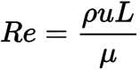
• R_e is the Reynolds number
• ρ is the density of the fluid (kg/m³)
• V is the velocity of flow (m/s)
• L is the pipe length (m)
• μ is the viscosity of the fluid (kg/m.s)
• When viscous forces are dominant, the flow is laminar.
• When inertial forces are dominant over viscous forces, the flow is said to be turbulent.
• Critical Reynolds number - It is associated with laminar-turbulent transition, where laminar flow becomes turbulent.

• In this challenge, you are required to do a literature review of various turbulence models explained in the Turbulence modeling video and explain why DNS isn’t feasible according to Kolmogorov's scale.
• There are two main phenomenon associated with turbulence , which is energy dissipation and noise generation.   
• Eddy formation in turbulent flow - Eddy is the movement of a fluid that deviates from the general flow of the fluid. An example of a vortex is a vortex that creates such a deviation. 
• Turbulent flow is defined .as flow in which the inertial forces of the system are dominant over the viscous forces. This phenomenon is described by the Reynolds number, a unitless number used to determine when turbulent flow occurs. Conceptually, the Reynolds number is the ratio between inertial forces to the viscous forces.
• Turbulent flow is highly stochastic.
• Laminar flow is observed at the initial stage of the boundary layer.
• At critical reynolds number , vortices formation starts .Large eddies break into smaller eddies ,after gaining enough energy.
• Sometimes smaller eddies coalese to form larger eddies as well. This process is called energy cascading.
• Mean flow is  the energy source for the large eddies. 
• Large eddies are the energy source for the small eddies.
• Unsteady, irregular (aperiodic) movement in which transported quantities (mass, momentum, scalar species) vary in time and area.
• Identifiable swirling styles signify turbulent eddies.
• Statistical averaging effects in responsible, turbulence related shipping mechanisms.
• This feature lets in for turbulence modeling,consists of a huge range of turbulent eddy sizes (scales spectrum).
  
  
• Types of Computational approach
• DNS -  Direct Numerical Simulation
• LES -  Large eddy simulation
• RANS - Reynolds Averaged Navier Stokes Simulation .

• DNS   - Direct Numerical Simulation  
• Direct numerical simulation (DNS)is a computational fluid dynamics (CFD) simulation in which the Navier–Stokes equations are solved numerically without any turbulence model. This means that the full range of spatial and temporal scales of turbulence must be resolved.
• Direct Numerical Simulation of Turbulence (DNS) has become a method of utmost importance for turbulence physics research, and its importance continues to grow due to the increasing popularity of high-performance computing techniques.
• DNS differs from conventional CFD in that turbulence is explicitly resolved, rather than modeled by a Reynolds-averaged Navier-Stokes (RANS) closure.

• LES -  Large eddy simulation
• Large eddy simulation (LES) is a mathematical model of turbulence used in computational fluid dynamics.
• It was originally proposed in 1963 by Joseph Smagorinsky to simulate atmospheric air currents and was first explored by Deardorff (1970). 
• The basic idea of ​​LES is to reduce the computational cost by ignoring the smallest length scales, which are the most computationally expensive to solve, using low-pass filtering of the Navier-Stokes equations. 
• Less expensive than DNS.
• Efforts and computational assets needed are still too large for most practical programs
  available in fluent.

• RANS - Reynolds Averaged Navier Stokes Simulation .
• The Reynolds-averaged Navier-Stokes equations (RANS equations) are time-averaged equations of motion for fluid flow.
• The idea behind the equations is the Reynolds decomposition, where an instantaneous quantity is decomposed into its time-averaged and fluctuating quantities.
• Idea first proposed by Osborne Reynolds.  
• To describe turbulent flows RANS model are used.

• The Spalart-Allmaras model 
• When in modified form, the eddy viscosity is easy to resolve near the wall. 
• Mainly intended for aerodynamic / turbomachinery applications with mild separation,such as supersonic /transonic flows over airfoils ,boundary layer flows etc.
• Embodies a relatively new class of  one equation  models where it is not necessary to calculate a length scale related to the shear layer thickness.
• Designed specifically for aerospace applications involving wall-bounded flows.
• Has been shown to give good results for boundary layers subjected to adverse pressure gradients.
• Gaining popularity for turbomachinery applications.

• The k- Epsilon turbulence models.
• Standard k-epsilon model
• The most widely used engineering turbulence model for industrial applications .
• Robust and reasonably accurate.
• Contains submodels for compressibility ,buoyancy , combustion,etc.
• Limitations - The epsilon equation contains a term which cannot be calculated at the wall. Therefore, wall functions must be used.
• Generally performs poorly for flows with strong separation,large streamline curvature, and large pressure gradient.

• Renormalization group(RNG) k-epsilon model.
• viscosity model to account for low Re effects.
• Analytically derived algebraic formula for turbulent prandtl/ Schmidt number.
• Swirl modification.
• Performs better than SKE for more complex shear flows, and flows with high strain rates, swirl and separation.     

• The k-omega turbulence models.
• The k-omega  family of turbulence models have gained popularity mainly because 
• The  model equations do not contain terms which are undefined at the wall that they can be integrated to the wall without using wall functions.
• They are accurate and robust for a wide range of boundary layer flows with pressure gradient.
• Fluent offers two varieties of k omega models.

 

• Standard k-omega(SKW) model
• Most widely adopted in the aerospace and turbo-machinery communities.
• Several sub-models/ options of k-omega; compressibility effects, transitional flows and shear flow corrections  

   

• Why DNS isn’t feasible according to Kolmogorov's scale.     
• Kolmogorov's theory describes how energy is transferred from larger to smaller eddies.
• How much energy are contained in eddies of a given size.
• How much energy is dissipated by vortices of each size.
• More time is needed to bond.
• Very fine meshes that result in more computing resources needed to run. Therefore, industries do not prefer this method as its inefficient.
• The challenge in turbulence modeling is the modeling of the eddies.
• Eddy is the swirling of a fluid and the reverse current created when the fluid is in a turbulent flow regime i.e when the flow around the body exceeds critical velocity. 
• Larger eddies break into smaller eddies on consuming smaller eddies
• Sometimes smaller eddies combine to form larger eddies This process is called energy cascading.
• Large eddies  size∝(LU∞)����∝(��∞) . Larger eddies gain energy from the mean flow.
• Small eddies size∝(LRe34)����∝(���34). Smaller eddies gain energy from large eddies.
• Kolmogorov's length scale is the smallest η=(ν3ε)14�=(�3�)14
• ε=
  (U3L)�=(�3�) is the rate of dissipation of turbulent kinetic energy. 
• Kolmogrov time scale tn=(νε)12��=(��)12, To detrmine turn over time of particular eddie)
• To check the feasibility of the DNS
• The ratio of the largest to the smallest eddies is given below

 
(Lη)=⎛⎝L(ν)34⎞⎠ε14

(Lη)=⎛⎝L(ν)34⎞⎠⎛⎝(u)34L14⎞⎠(��)=(�(�)34)((�)34�14)

(Lη)=⎛⎝L(u)34ν⎞⎠(��)=(�(�)34�)

(Lη)=Re34(��)=��34\

• To model the vortex they are divided into cells containing grids and this is easy for a large vortex.
• The same grid size is not useful for small vortex resolution, for smaller vortex we need to reduce the grid size.

• Procedure     
• Import the geometry model and create an enclosure.
• Meshing is done with the correct size and element size. Inlets, outlets and walls are used to name them.
• Then the boundary conditions are entered and the kW SST solver is selected. This model provides excellent results both near and far from the wall.
• Correct pressure and velocity planes and graphs are created to display the findings

       

         

        

• Meshing
• Element size = 1.253 mm

         

         

         

         

• Setup

      

      

• The model used: k-omega SST 

  The material used : air 

  Boundary condition : Inlet - velocity inlet = v = 60m/s

          

      

                    

• Pressure Contour

         

  

          

• Pressure streamline plot       

  

                   

        

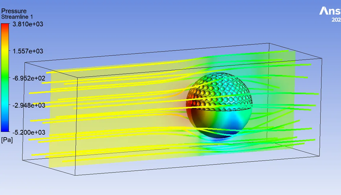
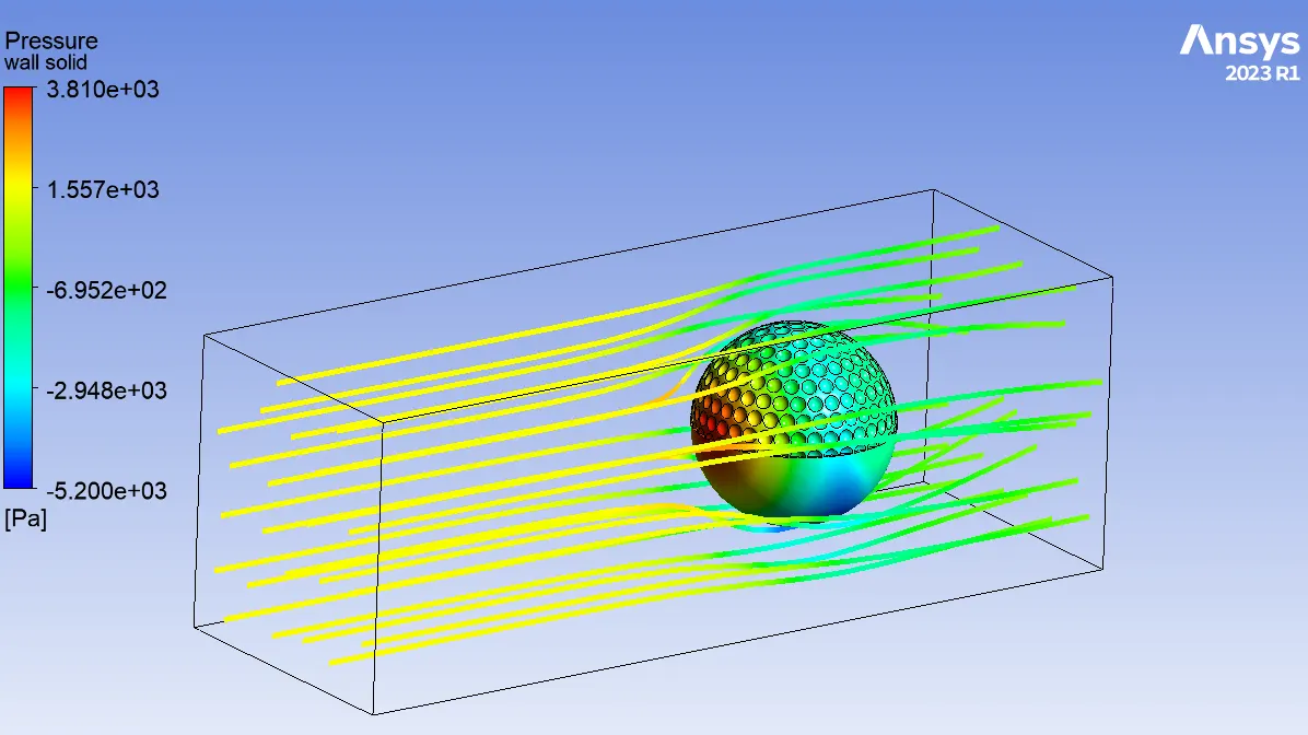
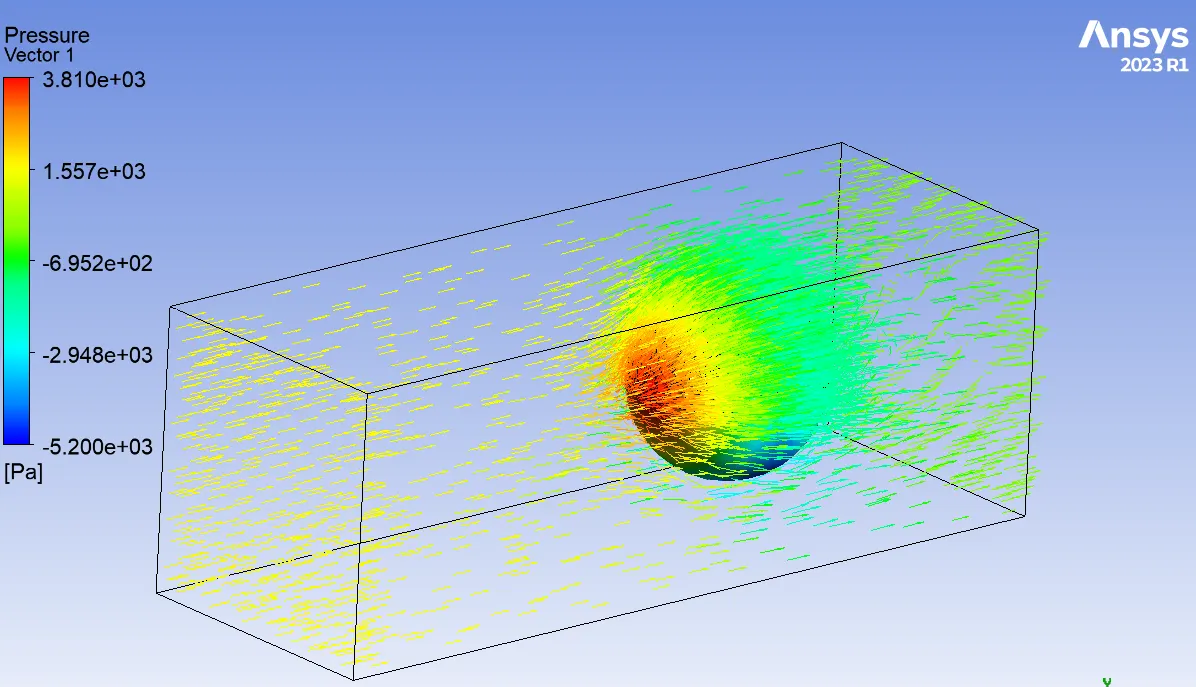
• Pressure Vector plot

          

• Velocity Contour 
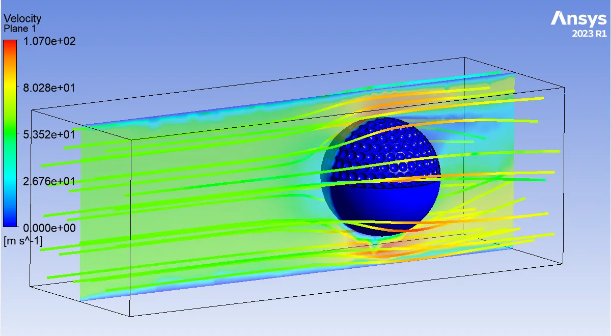
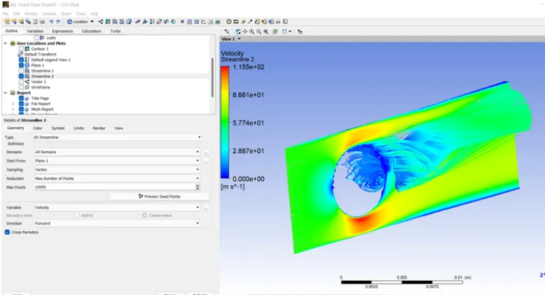
• Streamline Velocity contour

              

         

        

• Velocity Vector 
• From the velocity contour we conclude that ball will go downward.

          

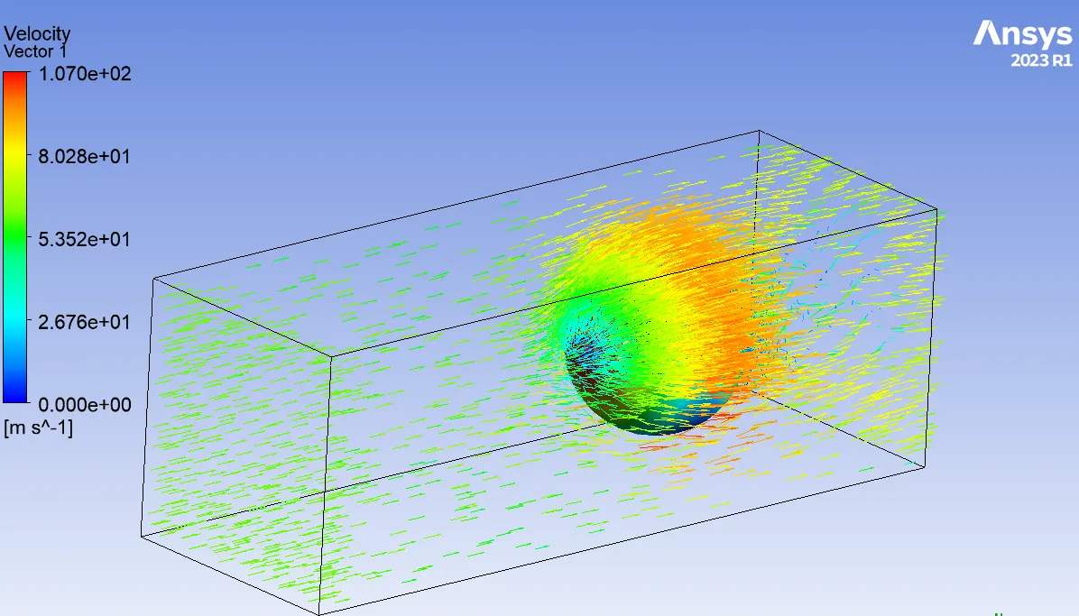
• The recirculation region helps the flow separating from the ball.
• In general, the term "wake" is used to describe any disturbance to the flow caused by an obstruction.
• Recirculation is a specific condition where the flow separates from the body of the obstacle. This creates a low-pressure region immediately downstream, which draws fluid back into that region from the main flow, with the net result of creating a circulating vortex or pair of vortices. This condition creates a significant increase in drag compared to situations where the flow remains attached to the surface.

• Conclusion
• From the velocity vectors we observed that the direction of the ball is moving down.
• The dimples of the golf ball serve to minimize drag by minimizing the wake (recirculation) area.
• It also helps with the flow attachment and tries to disconnect the flow from the golf ball.
• Therefore velocity of the flow beneath the  golf ball is high, resulting in low pressure and the formation of wake region following the rough surface.
• Air velocity on the smooth surface is higher, whereas the air velocity on the rough surface is lower. This causes a pressure difference which accounts for the balls downward swing.