Week 5 - Turbulence modelling challenge

TURBULENCE MODELLING ON A GOLF BALL

1 INTRODUCTION:

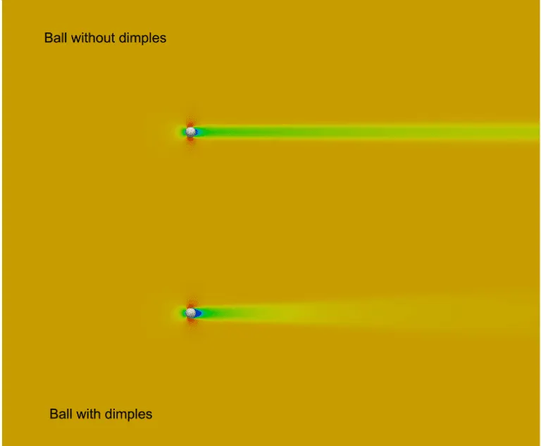
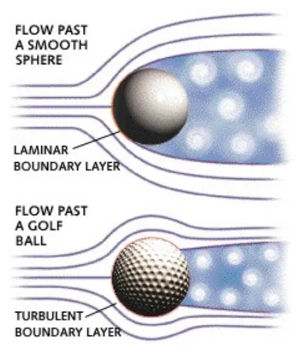
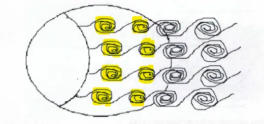
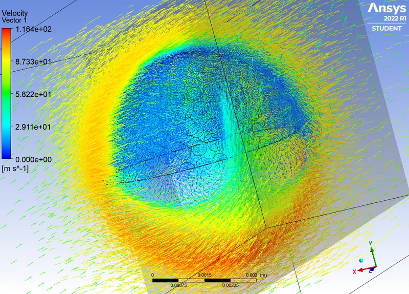
The aerodynamics of a golf ball is a complex study that has years of research in it. A smooth ball has a laminar flow around it. The fluid flow downstream detaches from the surface of the ball in the form of vortices. This is called flow separation, which gives rise to a viscous wake behind the ball that slows it down. After the aerodynamics of the ball study began, dimples were introduced in the ball's circumference. A Symmetric distribution of 300 - 500 dimples, with different geometry, is provided on the surface. The dimples act as artificial turbulators, creating turbulence next to the ball surface and creating to layers of air going around the ball. The top layer is going faster than the bottom layer. The air clings to the ball's surface, which creates turbulence. This reduces the drag and helps the ball to travel farther than a smooth one. The drag component, which is a result of the difference in the velocity of the solid and fluid body. It opposes the solid motion through the air. The lift component occurs when the fluid is turned by the solid, which creates an opposing force. If the ball spins in a way that pushes the air downward, then an upward lift force is experienced by the ball. This factor is seen when the ball is spinning. The spinning action makes the air pressure on the bottom of the ball higher than the air pressure on the top, and this imbalance creates an upward force on the ball. The final image shows the distribution of smaller eddies inside the dimple, which is separated from the outer surface of larger eddies. These smaller eddies cling to the surface, while the larger eddies are diffused to the fluid flow.

2 LITERATURE REVIEW:

2.1 TURBULENCE MODELS

To analyse various engineering flows in CFD applications, it is necessary to model the turbulent nature of the flow. Correct modeling of the turbulence directly converges to reliable results.

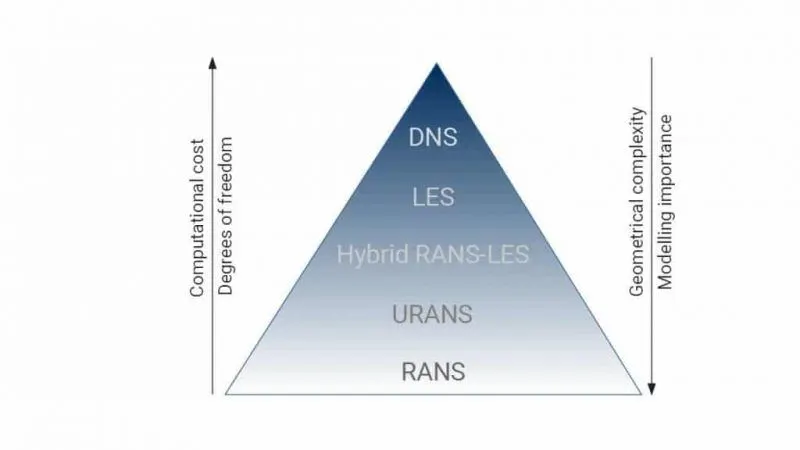
Turbulence causes the appearance in the flow of eddies with a wide range of length and time scales that interact in a dynamically complex way. Given the importance of the avoidance or promotion of turbulence in engineering applications, it is no surprise that a substantial amount of research effort is dedicated to the development of numerical methods to capture the important effects due to turbulence. The methods can be grouped into the following three categories:

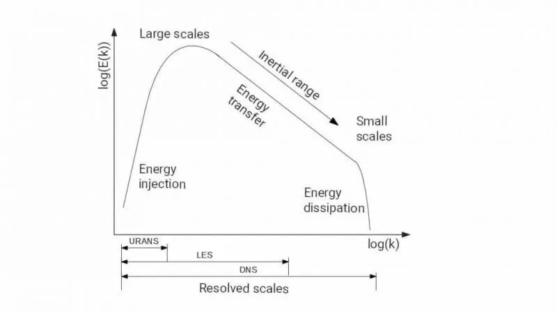
Direct numerical simulation (DNS): these simulations compute the mean flow and all turbulent velocity fluctuations. The unsteady Navier–Stokes equations are solved on spatial grids that are sufficiently fine that they can resolve the Kolmogorov length scales at which energy dissipation takes place and with time steps sufficiently small to resolve the period of the fastest fluctuations. These calculations are highly costly in terms of computing resources, so the method is not used for industrial flow computations.

Turbulence models for Reynolds-averaged Navier–Stokes (RANS) equations: attention is focused on the mean flow and the effects of turbulence on mean flow properties. Prior to the application of numerical methods the Navier–Stokes equations are time averaged (or ensemble averaged in flows with time-dependent boundary conditions). Extra terms appear in the time-averaged (or Reynoldsaveraged) flow equations due to the interactions between various turbulent fluctuations. These extra terms are modelled with classical turbulence models: among the best known ones are the k–ε model and the Reynolds stress model. The computing resources required for reasonably accurate flow computations are modest, so this approach has been the mainstay of engineering flow calculations over the last three decades.

Large eddy simulation: this is an intermediate form of turbulence calculations which tracks the behaviour of the larger eddies. The method involves space filtering of the unsteady Navier–Stokes equations prior to the computations, which passes the larger eddies and rejects the smaller eddies. The effects on the resolved flow (mean
flow plus large eddies) due to the smallest, unresolved eddies are included by means of a so-called sub-grid scale model. Unsteady flow equations must be solved, so the demands on computing resources in terms of storage and volume of calculations are large, but (at the time of writing) this technique is starting to address CFD problems with complex geometry.

Unsteady RANS Model (URANS):

RANS modelling is the most common and widespread approach in industrial applications. If the flow of interest is characterized by moving parts of periodic flow feature, these can be resolved using unsteady RANS (URANS)

Hybrid RANS-LES model:

There is a family of turbulence models where the benefits of LES modelling are being exploited while retaining the efficiency of RANS models where LES would be too expensive. These go under the name of hybrid RANS-LES models. The majority of the mesh resolution tends to be in proximity of surfaces and bodies of interest as in LES the flow needs to be fully resolved near the wall. The cost of LES can therefore be greatly reduced if the constraints of the increased resolution near the wall can be relaxed. One of the most common hybrid approaches uses LES modelling away from the walls and RANS modelling near the wall. This approach is called Detached Eddy Simulation (DES). The DES approach is becoming very popular in industrial applications as it helps overcoming some of the limitations of the RANS models as well as offering increased insight in the solution as the simulation is always run as unsteady flow, even for cases that have a steady state solution, and the finer spatial resolution allows to study detailed behaviour of the flow of interest. All of it at a reduced cost compared to a fully fledged LES approach.

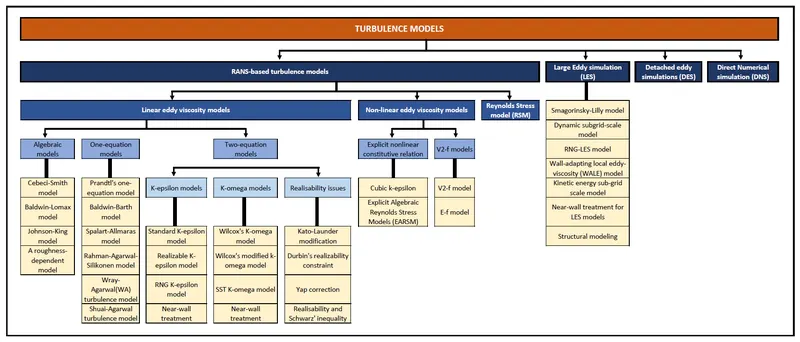
In order to be able to compute turbulent flows with the RANS equations it is necessary to develop turbulence models to predict the Reynolds stresses and the scalar transport terms and close the system of mean flow equations. For a turbulence model to be useful in a general-purpose CFD code it must have wide applicability, be accurate, simple and economical to run. The most common RANS turbulence models are classified on the basis of the number of additional transport equations that need to be solved along with the RANS flow equations.

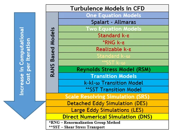
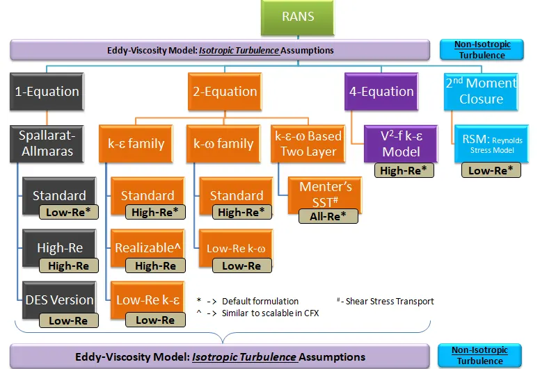
Few examples of turbulence models are:

2.2 KOLMOGOROV SCALE

Kolmogorov microscales are the smallest turbulent flow scales. Viscosity dominates and the turbulent kinetic energy is dissipated into heat, which is defined by Kolmogorov length, time and velocity scales.

Kolmogorov length scale, `eta = (v^3/epsilon)^(1/4)`

Kolmogorov time scale, `tau = (v/epsilon)^(1/2)`

Kolmogorov velocity scale, `u = (vepsilon)^(1/4)`

where `epsilon` is the average rate of dissipation of turbulence kinetic energy per unit mass, and `v` is the kinematic viscosity of the fluid. Typical values of the Kolmogorov length scale, for atmospheric motion in which the large eddies have length scales on the order of kilometers, range from 0.1 to 10mm; for smaller flows such as in laboratory systems, `eta` may be much smaller.

The Kolmogorov theory answers the questions of The size of the smallest eddies that are responsible for dissipating the energy. It also answers the phenomenon whether as l decreases, the characteristic velocity and timescales u(l) and `tau`(l) increase, decrease or stay the same. The assumed decrease of the Reynolds number by itself is not sufficient to determine these trends. So Kolmogorov's theory is based on three important hypotheses combined with dimensional arguments and experimental observations.

Kolmogorov's hypothesis of local isotropy states that at sufficiently high Reynolds number, the small-scale turbulent motions are statistically isotropic. Large scale turbulence may still be anisotropic.

Kolmogorov's first similarity hypothesis states that in every turbulent flow at sufficiently high Reynolds number, the statistics of the small scale motions have a universal form that is uniquely determined by `epsilon` and v.

Kolmogorov's second similarity hypothesis states that in every turbulent flow at sufficiently high Reynolds number, the statistics of the motions of scale 1 in the range lo>>l>>`eta` have a universal form that is uniquely determined by `epsilon` independent of v.

The Kolmogorov 1941 theory is a mean-field theory since it assumes that the relevant dynamical parameter is the mean energy dissipation rate. In fluid turbulence, the energy dissipation rate fluctuated in space and time. So it is possible to think of the microscales as quantifies that also vary in space and time. However, standard practice is to use mean-field values since they represent the typical values of the smallest scales in a given flow.

3 COMPUTATION OF A TURBULENCE CASE:

3.1 GEOMETRY PREPARATION

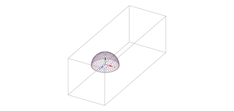
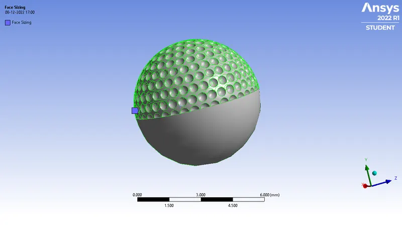
A symmetrical golf ball with standard dimples on one side and a smooth surface on the other side is made with an enclosure.

3.2 MESHING THE GEOMETRY AND DOMAIN

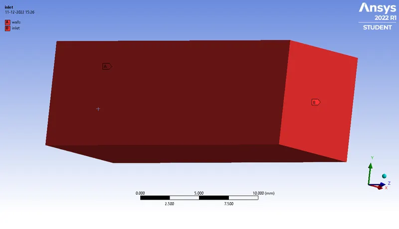
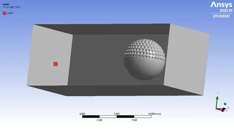
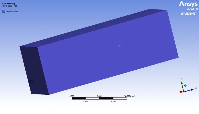
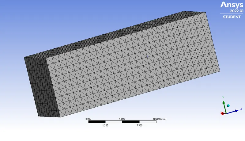
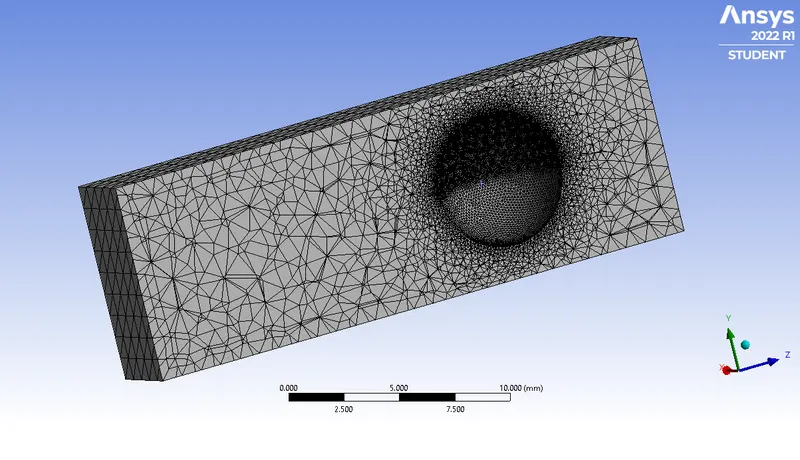
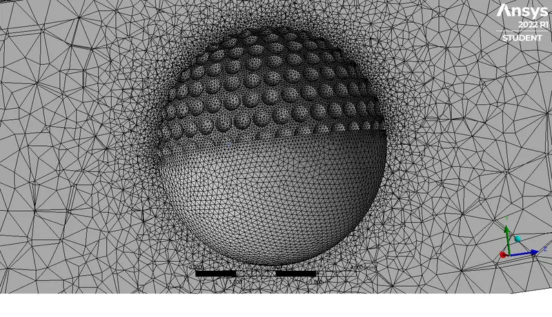
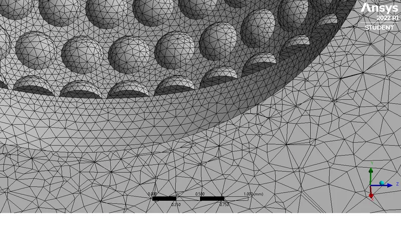
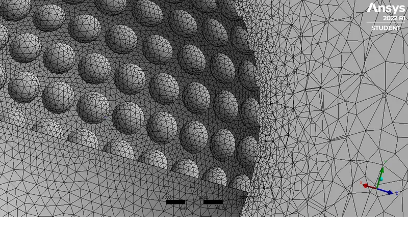
The inlet, outlet and the walls are named, with face meshing method on the walls, and size meshing is done on the dimples of the ball. The default element size is given as 1mm and the refined mesh around the golf ball is meshed with a size of 0.15mm.

3.3 SETTING UP THE SOLVER

3.3.1 Mesh checkup and general setup

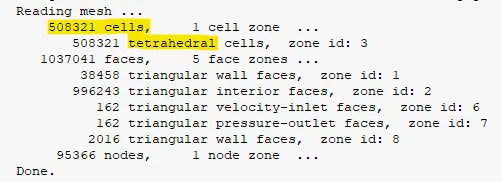
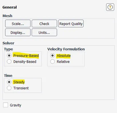
The mesh check is done and the general settings are set with a steady pressure-based solver.

3.3.2 Viscous model selection

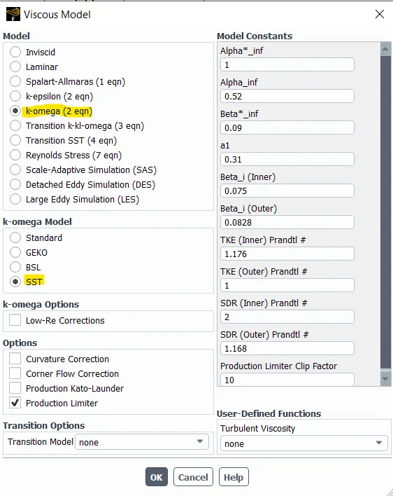
K-omega SST model is selected.

3.3.3 Boundary conditions and material selection

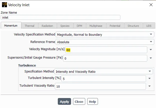
The air velocity is given at the inlet as 60 m/s, which is similar to the ball traveling in the opposite direction.

4 COMPUTATIONAL RESULTS:

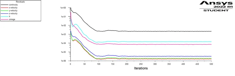
Solver convergence plot:

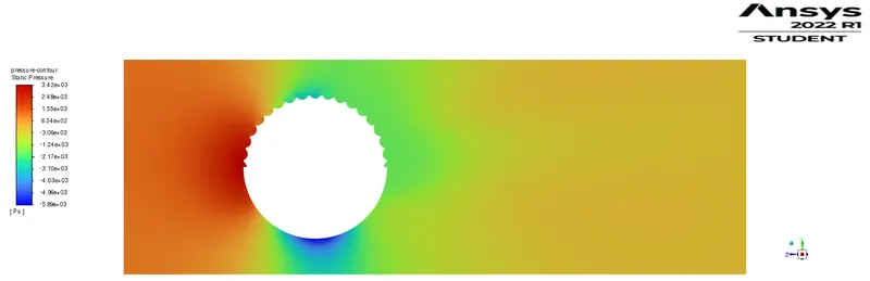
Pressure plot:

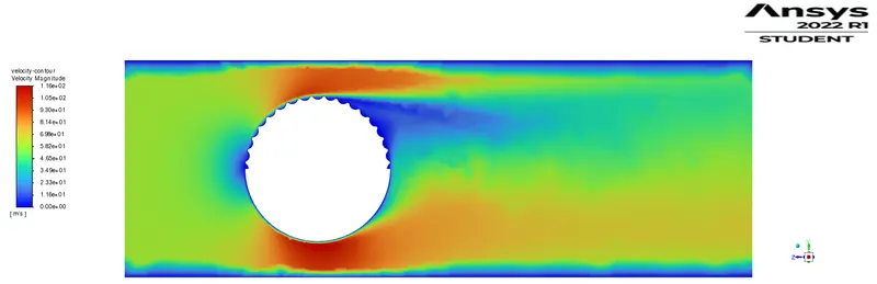
Velocity plot:

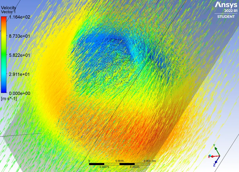
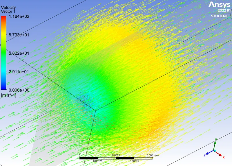
Velocity vectors:

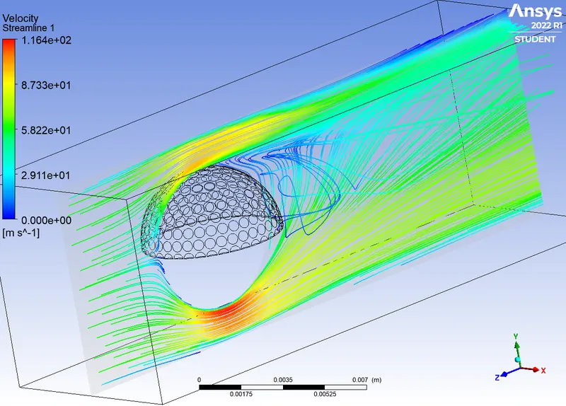
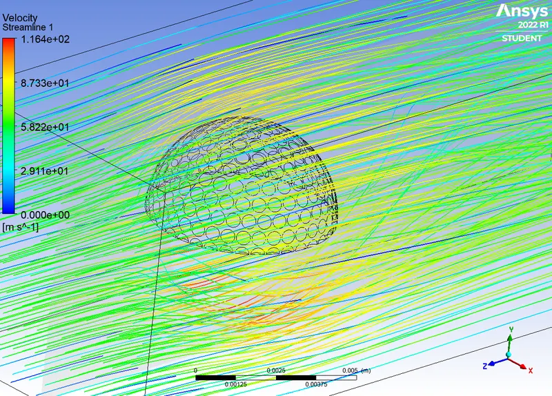
Stream lines:

5 INFERENCE:

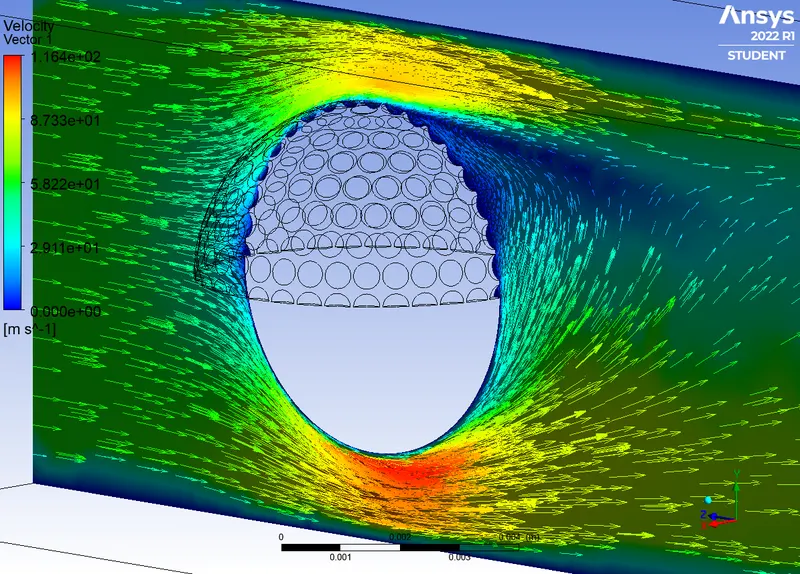
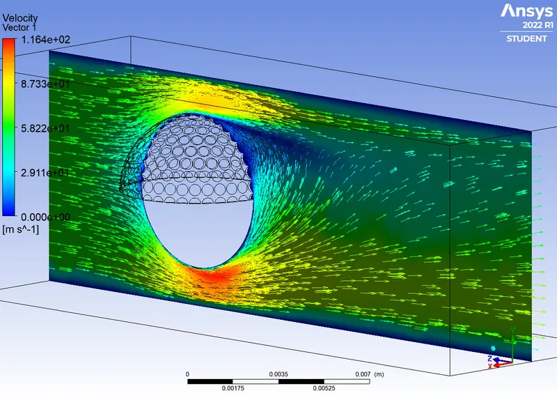
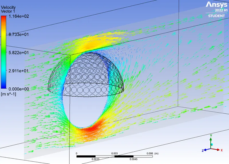
Aerodynamics of the golf ball: Based on the velocity and pressure plots, the aerodynamic behavior of the ball is evaluated. The ball has a symmetric geometry with respect to the two vertical axes. Hence there is no movement with respect to this axis. In aerodynamic terms, no yawing or rolling motion is observed on the body. Hence pitching motion is observed in the body, with the ball swinging or spinning towards the side with the dimples. The vector plot and streamline plot is a perfect illustration to represent the direction of motion. The vectors shows the movement of fluid particles around the ball surface which acts on the surface of the ball and in reaction, the ball moves aerodynamically.

The lift force can be anticipated from the velocity plot. Clearly there is high velocity gradient at the bottom of the ball which acts upwards. The pressure plot also shows a significant accumulation of pressure gradient which is concentrated at a certain point. The drag force is on the upper dimple side of the ball is significantly lower, since the boundary layer is small and the layer get split into smaller and larger eddies. While the smaller eddies get attached to the surface, the larger eddies get dispersed into the free stream. The phenomenon creates less drag at the upper half and more drag at the lower half. The drag on the upper side is less and the lift is acted upwards, which makes the ball swing towards the dimple side. The other axes motion are stationary since the geometry is symmetric on the two vertical axes.

The DNS Turbulence model is not feasible according to the Kolmogorov scale. Because DNS is not capable to predict results accurately compared with experimental measurements, in particular high Reynolds number viscous flow (Re>4000). The turbulent viscosity will be relevant. More work is needed to use turbulence model (RANS) related to practical applications. The DNS has no turbulent viscosity and no turbulence models in it and it requires a refining the mesh to capture the too small cells in the too agitated zones. The DNS is also very expensive in terms of computational time and memory.

6 CONCLUSION:

Thus the turbulence models have been studied by using a golf ball geometry. The aerodynamics of the ball is studied by using the velocity and pressure simulation in Ansys Fluent. The ball tends to swing towards the side with the dimples. A ball with dimples has about half of the drag compared to a smooth ball. The ball spin contributes to half of the lift, and the other half of the lift is provided by the golf ball dimples, which allows for the optimization of the lift force. Dimples with different geometry like circular, circular flat, circular shallow, hexagonal etc. are studied and developed in golf balls. The same effect on cricket balls is also studied.

7 REFERENCE:

[1] 5th Asia-Pacific Congress on Sports Technology (APCST); A study of golf ball aerodynamic drag; Firoz Alam*, Tom Steiner, Harun Chowdhury, Hazim Moria, Iftekhar Khan, Fayez Aldawi, Aleksandar Subic; School of Aerospace, Mechanical and Manufacturing Engineering, RMIT University, Melbourne, Victoria 3083, Australia. Received 8 April 2011; revised 15 May 2011; accepted 16 May 2011.

[2] Michalchuk, Walter Robert, "An Investigation of Different Golf Ball Dimple Flow Fields. " Master's Thesis,
University of Tennessee, 2006.