Week 5 - Turbulence modelling challenge

AIM:

To explain turbulence modelling and run a simulation for the Golf ball.

OBJECTIVE:

• Turbulence modelling.
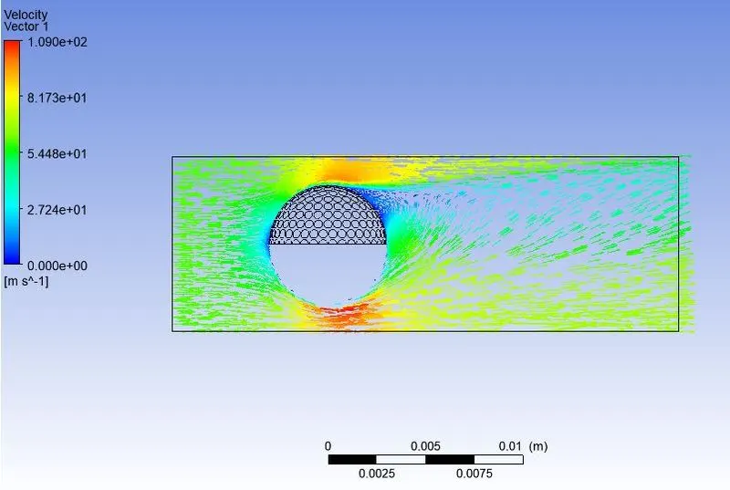
• To perform a 3D simulation and explain the recirculation region using velocity vectors.
• Visualize the wake region.

THEORY:

• Turbulence is unsteady, irregular fluid motion in which transported quantities (mass, momentum, scalar species) fluctuate in time and space.
• As of now, there is no sure-shot definition for turbulence. Some of the characteristics are:

1. Identifiable swirling patterns characterize turbulent eddies.

2. Enhanced mixing (matter, momentum, energy, etc.) results

3. Fluid properties and velocity exhibit random variations for this statistical averaging results in accountable, turbulence-related transport mechanisms.

Some of the turbulence models are :

A ) Zero Equation Model:

1. No PDE is used to solve the turbulent viscosity.

2. It fails to account for the transient behaviour of turbulent viscosity which leads to lower accuracy in results.

3. Directly solves turbulent viscosity using a Mixing length model.

4. Mixing length model assumes eddy viscosity terms to be dimensionally similar to two scales mainly Kolmogorov length scales & Kolmogorov velocity scales.

B ) Spalart Allmaras Model (S-A model) (One Equation Model):

1. It uses one set of equations to solve the turbulent kinetic energy to obtain turbulent viscosity.

2. The derived turbulent viscosity is substituted into the RANS model to solve the turbulence.

3. This is specifically designed for internal & external flows when the flow is attached, but not good when flows with strong adverse gradients or detaching flows.

C ) Two Equation models:

The mainly used models are :

1. Turbulent Kinetic Energy & Turbulent Dissipation Rate (K-epsilon Model):

In this K-epsilon (k-ε) turbulence model is used to simulate mean flow characteristics for turbulent flow conditions. It is a two-equation model which gives a general description of turbulence using two transport equations (PDEs). The original impetus for the K-epsilon model was to improve the mixing-length model.

2. Turbulent Kinetic Energy & Specific Dissipation Rate (K-omega Model)

• It predicts turbulence by two partial differential equations for two variables, k and ω, with the first variable being the turbulence kinetic energy (k) while the second (ω) is the specific rate of dissipation.
• It is a widely used model industry: mainly in aerospace and turbomachinery.

DNS isn’t feasible according to Kolmogorov's scale:

1. It is a more tedious process for a solution to converge

2. It requires very fine meshes which results in more computational resources for a simulation to run. Hence industries don't prefer this method as its inefficient.

SETUP & SOLUTION:

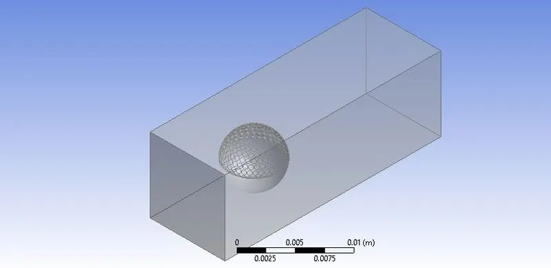
GEOMETRY:

• Import the geometry in fluent.

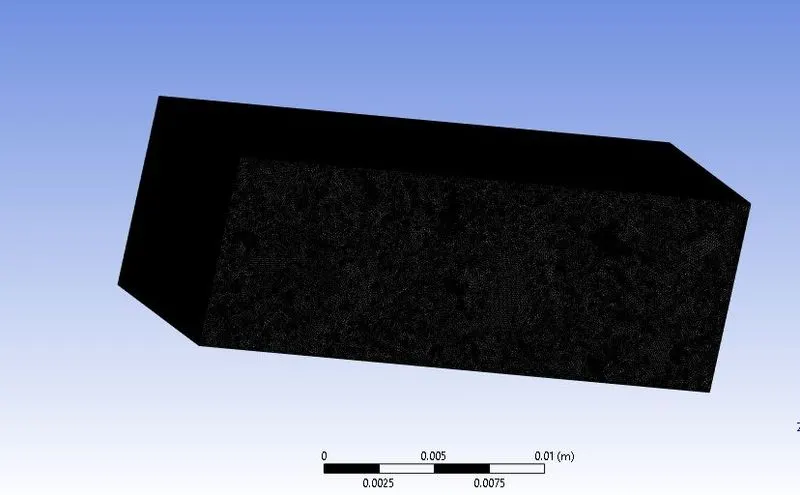
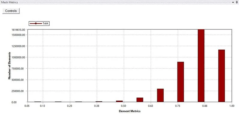
MESHING:

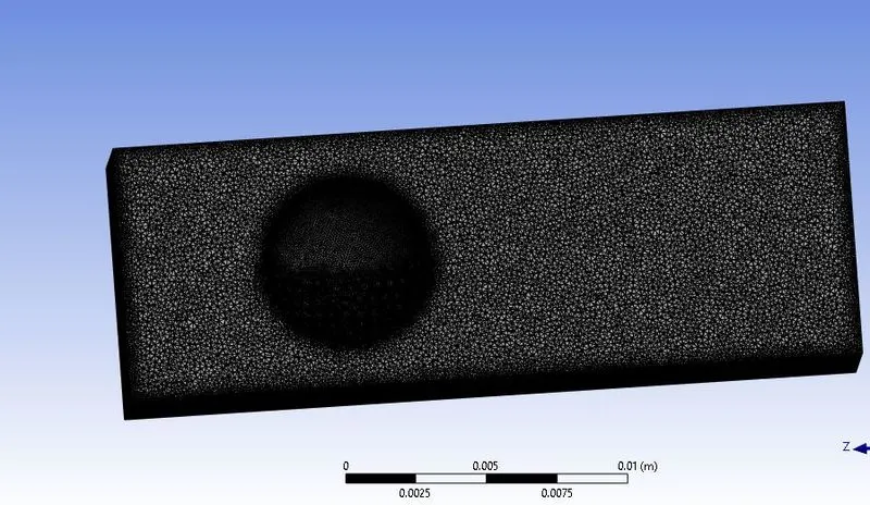
• The element size was given as 0.0001m and the meshing accordingly as input and output.

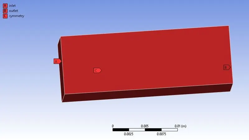
• Naming selection,

• Mesh cross-section,

• Setup:

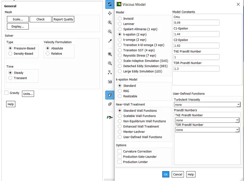
• Pressure-based - K-epsilon method

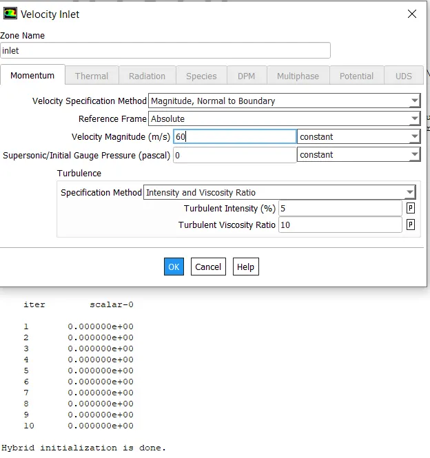
• Inlet - 60m/s.

• Hybrid initialisation is done.

RESULT:

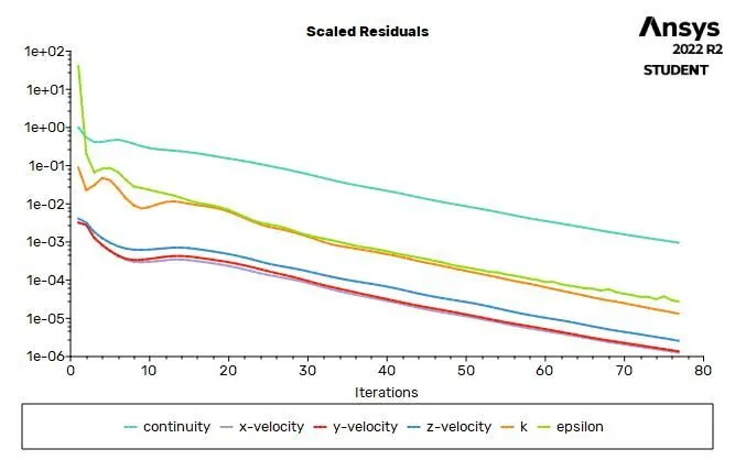
RESIDUAL:

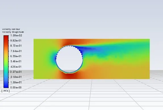
• Velocity Contour:

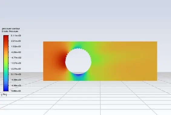
• Pressure contour:

• Velocity-Vector plot:

CONCLUSION:

• After observing the velocity vectors the direction of the ball is it's going down and the dimples on the golf ball help to reduce the drag by reducing the wake region. It also helps the flow to be attached and tries to separate the flow away from the golf ball.
• The wake region behind the ball is captured.
• Simulated an external flow around a sphere with dimples
• Extracted contours.