Week 5 - Turbulence modelling challenge

Challenge Description :

1. In this challenge, you are required to do a literature review of various turbulence models explained in the Turbulence modelling video (Week-5) and explain why DNS isn’t feasible according to Kolmogorov's scale.
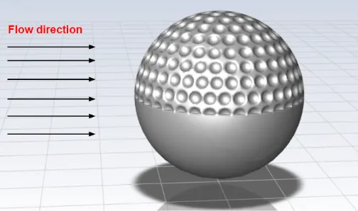
2. For the below geometry performs a 3D simulation and explains the recirculation region using velocity vectors.
3. Consider the flow direction of air, the ball is travelling opposite to it at 60m/s. Explain in which direction the ball will curve by visualising the wake region.

Answer:

Part 1: Explain different turbulence models & why DNS isn’t feasible according to Kolmogorov's scale.

There are two main models are available to model turbulence which are as follows:

1. First Order Models:

First order models assume analogy between laminar & turbulent flows. They assume that the average turbulent flow field is similar to the laminar flow field which results in lower accuracy.

It has three subtypes of models based on the number of equations the model is solving.

- Zero Equation Models

- One Equation Models (Spalart Allmaras model)

- Two Equations Models (K-epsilon model & k-omega model)

2. Second Order Models:

These models are solving the transport equations additionally to derive Reynolds stress terms in 3D.

As these models are solving additional equations to work in 3D & also PDEs are of the 2nd order, it has the highest accuracy but computationally very expensive. And because of large number of extra equations, these models are sensitive to boundary conditions as well. These models are commonly used in the industries.

This type also has subtypes.

- Algebraic Stress Model

- Reynolds Stress Model

The main difference between first order & second order model is that first order model uses the PDEs of 1st order to derive Reynolds stress terms while the second order models are using the PDEs of 2nd order because of that the accuracy of the second order models are more than the first order models but computationally more expensive.

Detail explanation of each model of First Order Models are as follows:

Zero Equation Model:

- No PDE is used to solve the turbulent viscosity.

- Fails to account for transient behaviour of turbulent viscosity which leads to lower accuracy results.

- Directly solves turbulent viscosity using a Mixing length model.

- Mixing length model assumes eddy viscosity terms to be dimensionally similar to two scales: Kolmogorov length scales & Kolmogorov velocity scales

One Equation Model:

- This model uses one set of equations to solve the turbulent kinetic energy in order to obtain turbulent viscosity.

- The derived turbulent viscosity is substituted into the RANS model to solve the turbulence.

- Spalart Allmaras Model (S-A model) is one eqation model. This S-A model is specifically designed for internal & external flows when the flow is attached, but not good when flows with strong adverse gradient ot detaching flows.

Two Equation models:

These models solve two PDEs to determine following quantity based on the model used.

- Turbulent Kinetic Energy & Turbulent Dissipation Rate (K-epsilon Model)

- Turbulent Kinetic Energy & Specific Dissipation Rate (K-omega Model)

K - epsilon Model:

This model has three different variants:

(a) Standard k-epsilon model:

- This is the most widely used model in the industries.

- It uses wall functions to calculate epsilon near wall.

- It is very known model to have very good convergence & memory efficient characteristics.

- It is very good model for attached & turbulent flows and also for solving external flow around complex bodies.

- This model performs very poorly for seperated flows.

(b) Realizable K-epsilon Model:

- Realizable & RNG types of K-epsilon models modify the existing epsilon equations to detemine Reynolds Stress terms.

- It solves some of constraints on Reynolds stresses.

- It shows consistent results with physics of turbulent flows.

(c) Renormalized Group (RNG) K-epsilon Model:

- This model uses the renormalized group theory to improve the epsilon equations.

- The effect of swirl in turbulent flow introduced using this model.

- It uses empirical relations to find a modified version of Prandtl Number to determine turbulent viscosity.

k-omega Model:

- It is very popular model in industry.

- This model does not contain terms that are defined at the wall. Hence, wall functions are not required at the wall to capture turbulence flows.

- It has two types of variants: one is Standard K-omega model & the other is SST K-omega model.

(a) Standard K-omega model:

- It is widely adopted in aerospace & turbomachinery components.

(b) SST (Shear Stress Turbulence) K-omega model:

- It is go-to model in all the other industries than the aerospace & turbomachinery.

- SST model uses a blending functions to transition from standard k-omega model to a higher Reynolds model away from the wall to better approximate turbulent flows.

Part 2:

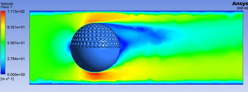
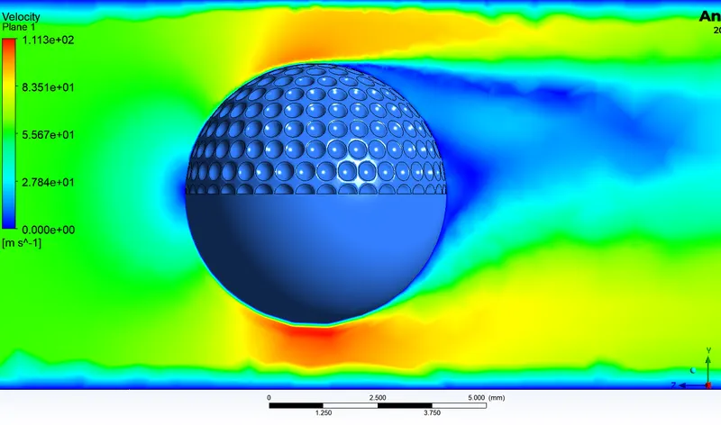
Objective is to determine which way ball is going to move. The velocity contour graph & vector plot will be presented.

Inputs: Air velocity: 60 m/s

Following model has been received as input:

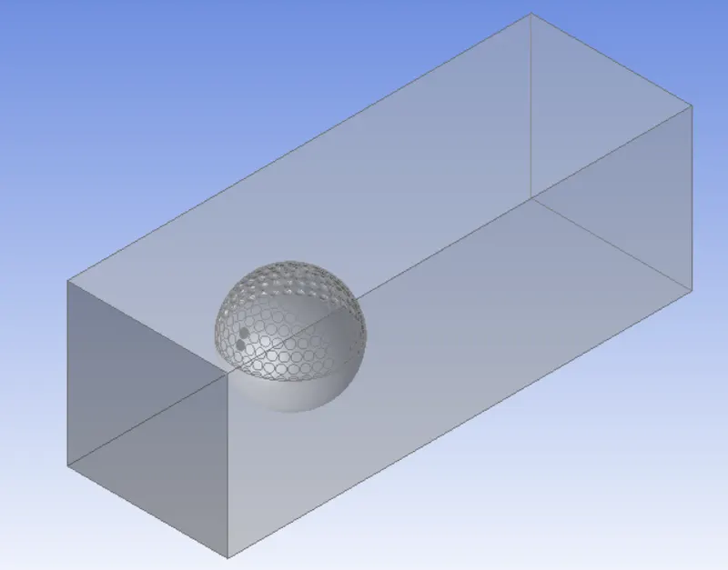
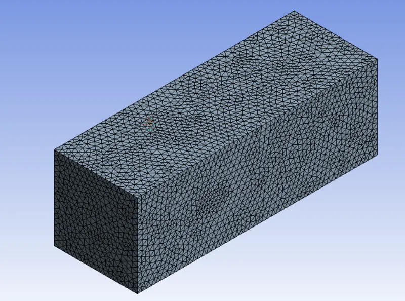
Mesh Model:

Element length: 0.75 mm

Number of Elements: 485872

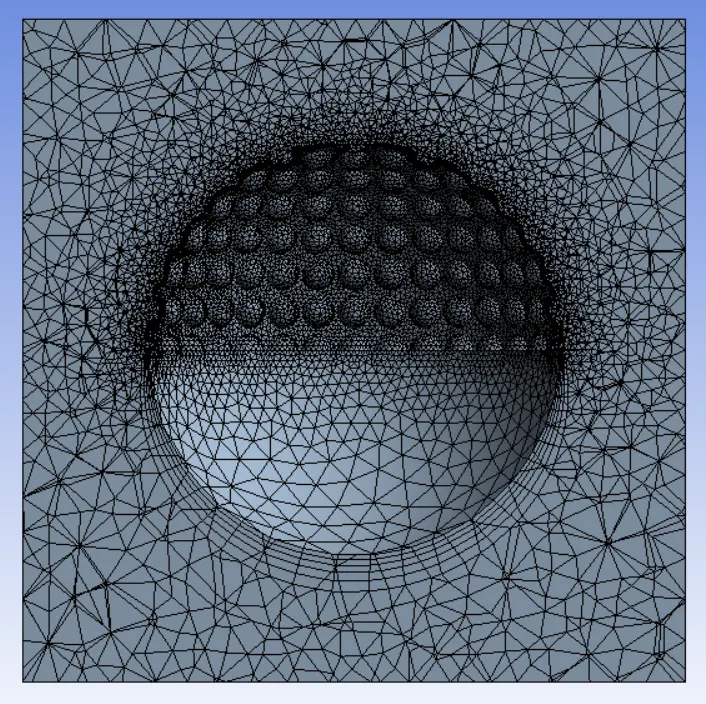
cross section of the model to visualize the generated mesh near the golf ball.

Turbulence Model used for the simulation: SST K-omega Model

Material: Air

Inlet: 60 m/s

Initialization: Standard

Iterations: 300

Results:

CFD-post has been used for post-processing the simulation results.

Velocity Contour Plot:

Velocity vector plots:

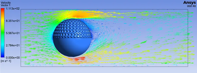
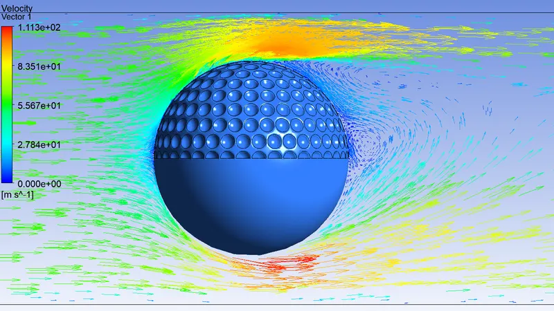
Velocity Streamline Plot:

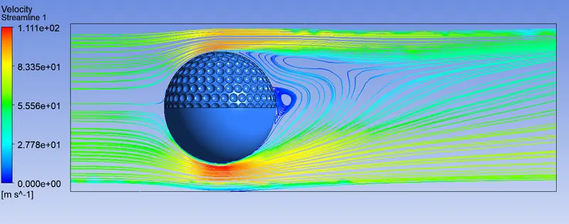
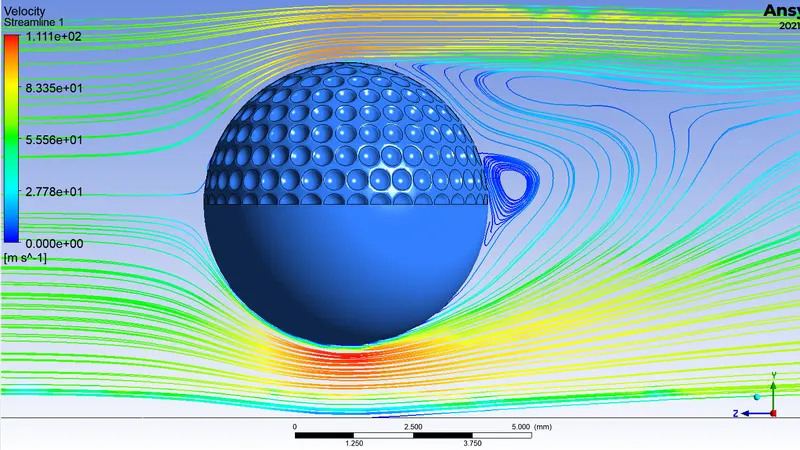
From above vector plot, it can be said that the ball will curve downward. The wake region or recirculation region at the back side of ball shows the direction of arrow circulating downward.

The recirculation region also helps the flow seperating from the ball.