Week 5 - Rayleigh Taylor Instability
Model & Simulation Setup Process:
The model has been created in Ansys Spaceclaim. Two square with 20mm X 20mm has been created which will represent water & air respectively.
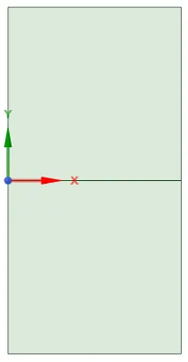
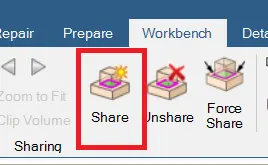
Shared topology has been created using following option.
The mesh has been generated using Ansys Mesh workbench by applying 0.5mm element size for baseline case & 0.4mm for refined case.
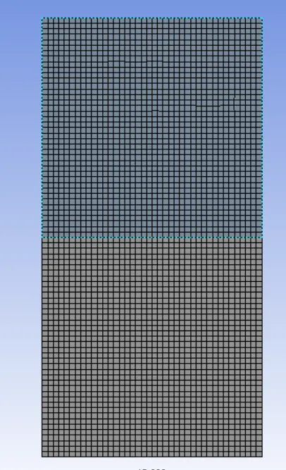
For the first square, water side name has been given while the bottom one has been given as air side.
In Simulation setup, default materials (air & water) has been used for first case & user defined material has been used for second case with given material properties.
- Laminar turbulence model has been used because of very low velocity.
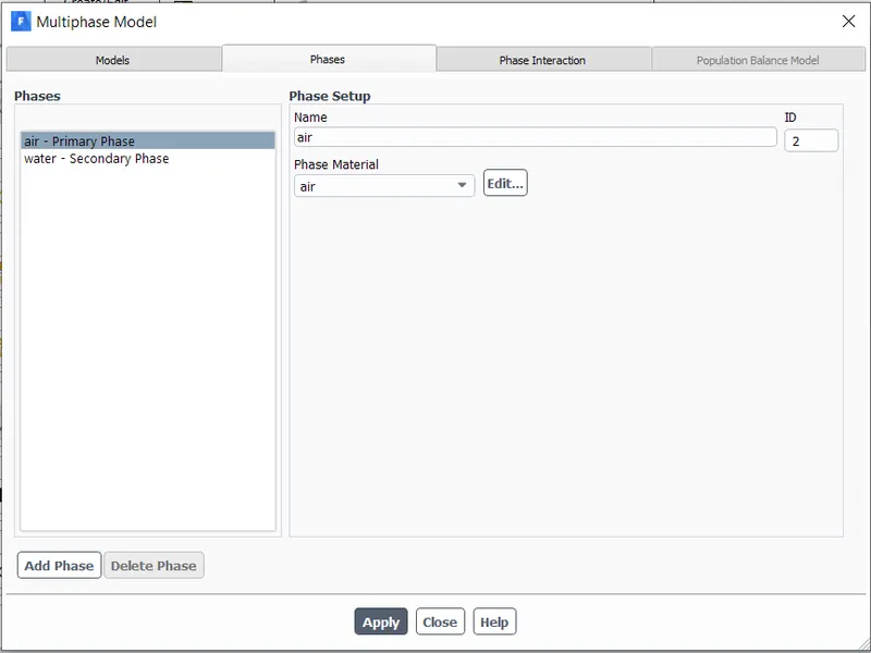
- In Multiphase Model setup dialogue box, volume of fraction has been chosen as homogeneous model while implicit formulations has been volume fraction. Two eulerian phases has been created, each for water & air or uder defined material. In Eulerian phase, the fluid is assumed to be incompressible, isothermal & newtonian fluid.
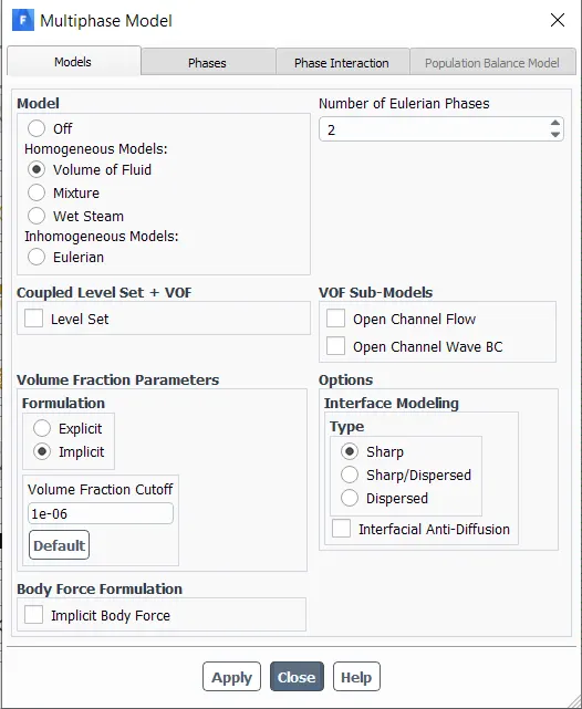
In the phases sectionin above dialogue box, the name has been given to each phase.
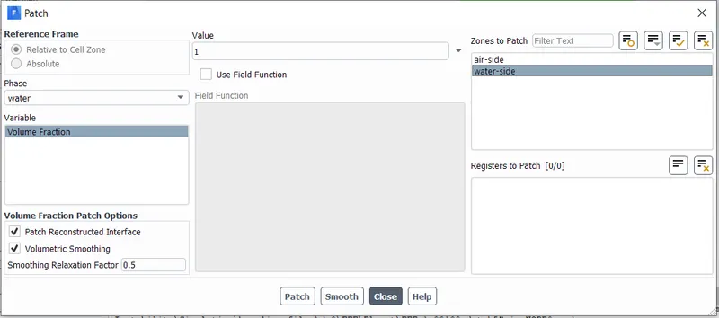
- In next step, standard initialization has been initiated. After that Patch has been performed between two phases. The patch for water has been shown in below window which indicates in the water side section, there is no air by indicating "1" and in the similar way, the air side has no water by indicating "0" in value section.
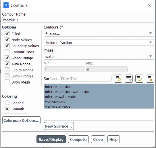
The contour graph to capture the water & air phases & animation for the simulation has been setup. After these, time step size & number of time steps has been inserted & simulation has been solved.
Q & A:
1. What are some practical CFD models that have been based on the mathematical analysis of Rayleigh Taylor waves? In your own words, explain how these mathematical models have been adapted for CFD calculations.
- Following CFD models are based on the Rayleigh-Taylor waves:
a) Kevin-Helmoltz (KH) Instability - It typically occurs between two immiscible fluids with a velocity difference accross their interface. This instability can be observed, for example, as a natural phenomenon of certain cloud patterns. These patterns are characterized by the generation of small-scale motion at the interface. which later leads to the formation of an unstable interfacial vortex street. This generates spiral structures at the fluid-fluid interface. Wave formation on still water due to blowing wind is another common example of instability.
b) Plateau-Rayleigh Instability - It is called the Rayleigh Instability & also related to Rayleigh - Taylor Instability. It explains why & how a falling stream of fluid breaks up into smaller packets with the same volume but less surface area. This model is a part of a greater branch of fluid dynamics concerned with fluid thread breakup.
c) Richtmyer - Meshkov Instability (RMI) - It occurs when two fluids with different density are impulsively accelerated because of the passage of shock wave. The development of the instability begins with small amplitude perturbations which initially grow linearly with time. Ans this is followed by a nonlinear regime with bubbles appearing in the case of a light fluid penetrating a heavy fluid and spikes appeari in the case of a heavy fluid penetrating light fluid. A chaotic regime eventually is reached and the two fluids mix. This instability can be considered the impulsive-acceleration limit of the Rayleigh - Taylor instability.
2. Perform the Rayleigh Taylor instability simulation for 2 different mesh sizes with the base mesh being 0.5 mm. Compare the results by showing the animations( Attach them from your google drive). Observe the differences in the animation and explain the effect of mesh size on simulation. Also, explain why a steady-state approach might not be suitable for these types of simulation.[ Choose Air and Water for this simulation]
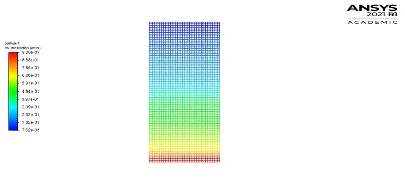
- Results for the base mesh with 0.5 mm element size are as follows:
Contour graph has been created using following option.
Contour Graph:
Animation:
- Results for refined mesh with same model & simulation setup but with improved mesh
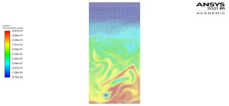
Contour Graph:
Animation:
In first simulation baseline mesh has been created using 0.5mm element size while for refined mesh 0.4 mm has been used. The refined mesh has been created using 0.1 mm & 0.25mm initially, but "floating point exception" error has occurred. The time step size has also been changed from 0.025 sec to 0.001 sec & 0.05 sec but same error has been faced. At last simualtion has been successfully performed using 0.4mm element size & 0.025 sec time step size.
The rayleigh taylor instability has been seen at the intereference of air & water while higher density fluid (Water) is moving down under gravity effect & low density fluid (air) is moving upwards. In this movement of fluids, vortex & fluid bubbles were created which can be seen in both animation videos.
And second point, the refined mesh will be needed more iterations compare to baseline base. In baseline mesh, the water has bee stabilized at the bottom before even completing the number of iterations, while in refined mesh still water has been moving down & has not been stabilized.
By increasing element size, more details has been captured and gravity effect on the water has been captured more precisely. The difference can be seen more effectively by comparing animation videos attached for both setup. Both vortex & fluid bubbles can be observed at the centre more effectively than the first case.
- In this type of simulation, the fluid movement will be captured with respect of time & in steady state simulation, captureing this movement is not possible.
3. Run one more simulation with water and user-defined material(density = 400 kg/m3, viscosity = 0.001 kg/m-s) for refined mesh.
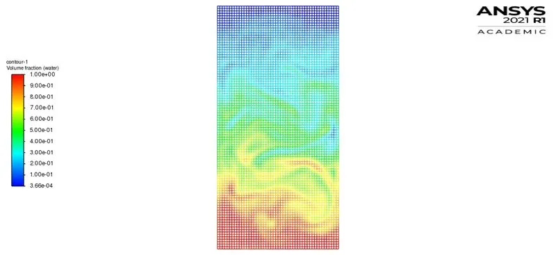
The user defined material has been created using the given material properties. The results of this simulation is as follows:
Time step size: 0.025 sec
No. of time steps: 200
Element size: 0.4 mm
Contour Graph:
Animation:
4. Define the Atwood Number. Find out the Atwood number for both the cases and explain how the variation in Atwood number in the above two cases affects the behavior of the instability.
- Atwood number is used in fluid dynamics to study hydrodynamic instabilities in density stratified flows and it is dimensionless number. It can be defined using following formula:
`A = (rho1 - rho2)/(rho1 + rho2)`
where, `rho1 =` density of heavier fluid
`rho2 =` density of lighter fluid
It is especially important in Rayleigh- Taylor instability because it helps to understand penetration distance of heavy fluid bubbles into the light fluid which is function of acceleration time scale, Agt^2 where g is gravitational force & t is the time.
It will help in detemining the fluid flow state in case of any disturbance.
To distinguish between the different states of fluid flow one must consider how the fluid reacts to a disturbance in the initial state. These disturbances will relate to the initial properties of the system, such as velocity, pressure, and density.
The concept of stable and unstable flow:
For a stable flow, any infinitely small variation, which is considered a disturbance, will not have any noticeable effect on the initial state of the system and will eventually die down in time. For a fluid flow to be considered stable it must be stable with respect to every possible disturbance. This implies that there exists no mode of disturbance for which it is unstable.
On the other hand, for an unstable flow, any variations will have some noticeable effect on the state of the system which would then cause the disturbance to grow in amplitude in such a way that the system progressively departs from the initial state and never returns to it. This means that there is at least one mode of disturbance with respect to which the flow is unstable, and the disturbance will therefore distort the existing force equilibrium.
- Calculating Atwood number for both cases:
for first case of air & water,
A = (998.2 - 1.225) / (998.2 + 1.225) = 0.9975
for second case of water & uder defined mateial,
A = (998.2-400)/(998.2+400) = 0.42
From above calculation & observing the results of both cases, it is clear that first case has achieved the stability after getting disturbed but in case of second simulation, the flow became unstable and never get back to its original states which means it is unstable flow.