Week 5 - Rayleigh Taylor Instability

Objective:-

To perform Rayleigh Taylor instability simulation for three different mesh sizes and compare the animations.

1. To develop a numerical case set-up for Raleigh-Taylor instability problem in Ansys Fluent.
2. To conduct grid independency test to understand the variation in RT instabilities.
3. To understand the effect on RT instabilities due to variation in Atwood number.

Introduction:-

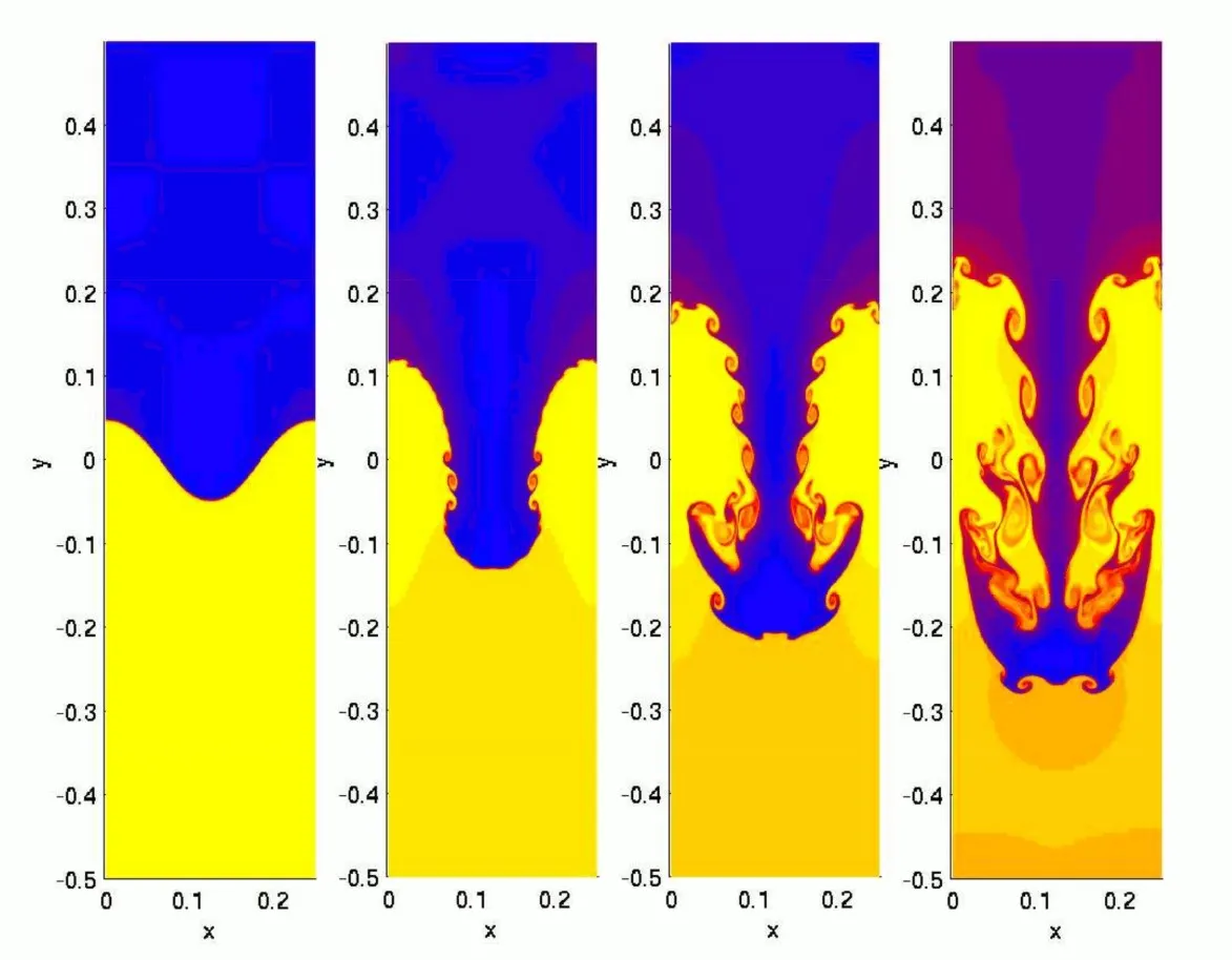
Rayleigh-Taylor Instability(RTI) is a hydrodynamic instability that occurs when a lighter fluid pushes against a heavier fluid. CFD is a branch of fluid mechanics that uses numerical analysis to simulate fluid flows.

Examples:-Water suspended above oil, Mushroom cloud from volcanic eruptions, supernova explosions, and instabilities in plasma fusion reactors.

Transient Simulation:-

• Transient simulations are performed to capture the mixing of fluids at various intervals.
• Transient simulation is more accurate than steady state simulations because it's a time marching solution.
• Transient simulation can capture instabilities by using smaller time steps.
• The interface thickness has a significant impact on numerical diffusion.
• The Variation of Atwood number has a direct impact on the perturbation amplitude and evolution of interface growth.
• Smaller time steps are required to observe and capture the instabilities.

Mathematical Analysis of Rayleigh-Taylor waves:-

Mass diffusion model:-

The mass diffusion equation describes the transport of mass and energy due to model viscosity and hence drives actual mixing in the fluids. Even if any configuration is Rayleigh-Taylor unstable, the diffusion process could be responsible for significant mixing if the viscosity is sufficiently large.

Single Fluid model:-

1. Potential flow model:-

This model is valid for all instability changes from the very linear stage through the early non-linear but limited to Atwood number of 1.in this model, the single mode perturbation expands, the flow equation to second order around the bubble tips, hence obtaining an ordinary differential equations for the bubble velocity.

2.Buoyancy drag model:-

It is valid for every Atwood number but limited to non-linear stages of the instability. it uses ordinary differential equations to evolve the width of the mixing layer. The bubble, spikes or amplitudes are described by balancing the inertia, buoyancy and drag forces. This model cannot deal with multiple mixing interfaces; can't be easily extended to two or three dimensions, and as a rule , do not address de-mixing, also known as counter gradient transport i.e. reduction of total fluid masses within the mixing zone. To address the above problems , two-fluid(multi-fluid) models has to be used.

3.Besnard-Harlow-Rauenzahn(BHR):

Its is more advanced version of the single -fluid model. The BHR model is based upon the evolution equations arising from second-order corrections and gradients-diffusion approximations. using a mass weighted-averaged decomposition, the original BHR model includes the full transport equation for the Reynold's stresses, turbulent mass-flux velocity, density fluctuations and turbulent kinetic energy dissipation rate.

Multi-fluid models:-

These models use a separate set of equations for each fluid in addition to the main flow equations and provide an accurate modeling de-mixing by correctly capturing the relative motion of different fluid fragments.

Two equations k-L turbulence model:-

The K-L turbulence model involves equation for turbulent kinetic energy(k) and turbulent length scale(L). The starting point for deriving the model equations are the buoyancy-drag models for the self similar growth for RT instabilities.

Kelvin-Helmholtz instability:-

The Kelvin-Helmholtz instability can occur when there is a velocity shear in a single continuous fluid or when there is a velocity shearing in a single continuous fluid or a velocity difference across the interface between two fluids. Kelvin-Helmholtz instabilities are visible in the atmosphere of plants and moons, such as in cloud formation on earth on the road spot on Jupiter, and the atmosphere of the sun and other stars.

Richtmyer-Meshkov instability:-

The Richtmyer-Meshkov instability (RMI) occurs when two fluids of different density are impulsively accelerated. Normally this is by the passage of a shock waves. The development of the instability begins with small amplitude perturbations which initially grow linearly with time. This is followed by a nonlinear regime with bubbles appearing in the case of a light fluid penetrating a heavy fluid, and with spikes appearing in the case of a heavy fluid penetrating a light fluid.

Plateau-Rayleigh Instability:-

The Plateau-Rayleigh Instability, often just called the Rayleigh instability, explains why and how a falling stream of fluid breaks up into smaller packets with the same volume but less surface area. It is related to the Ryleigh-Taylor instability and is part of a greater branch design of a particular type of ink jet technology whereby a jet of liquid is perturbed into a steady stream of droplets.

Geometry:-

Click and drag Ansys fluent in Ansys workbench to create a new project and name it Rayleigh Taylor instability.

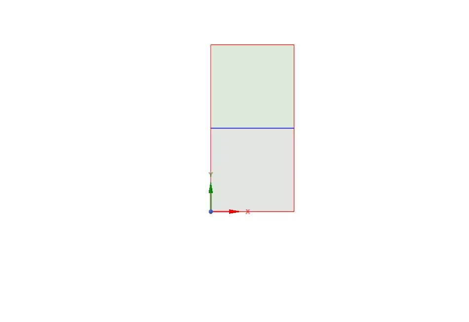
Double click on geometry to open the spaceclaim and now we have to create two squares of dimensions 20mm*20mm one upper and second one lower.

First create the lower volume and then extract it, then create the upper volume and then extract it.

Name the lower volume as Air and the upper volume as water, and then share the topology such that share one interface edge.(use 'shareprep' tool from workbench.) Now close geometry.

Case-1

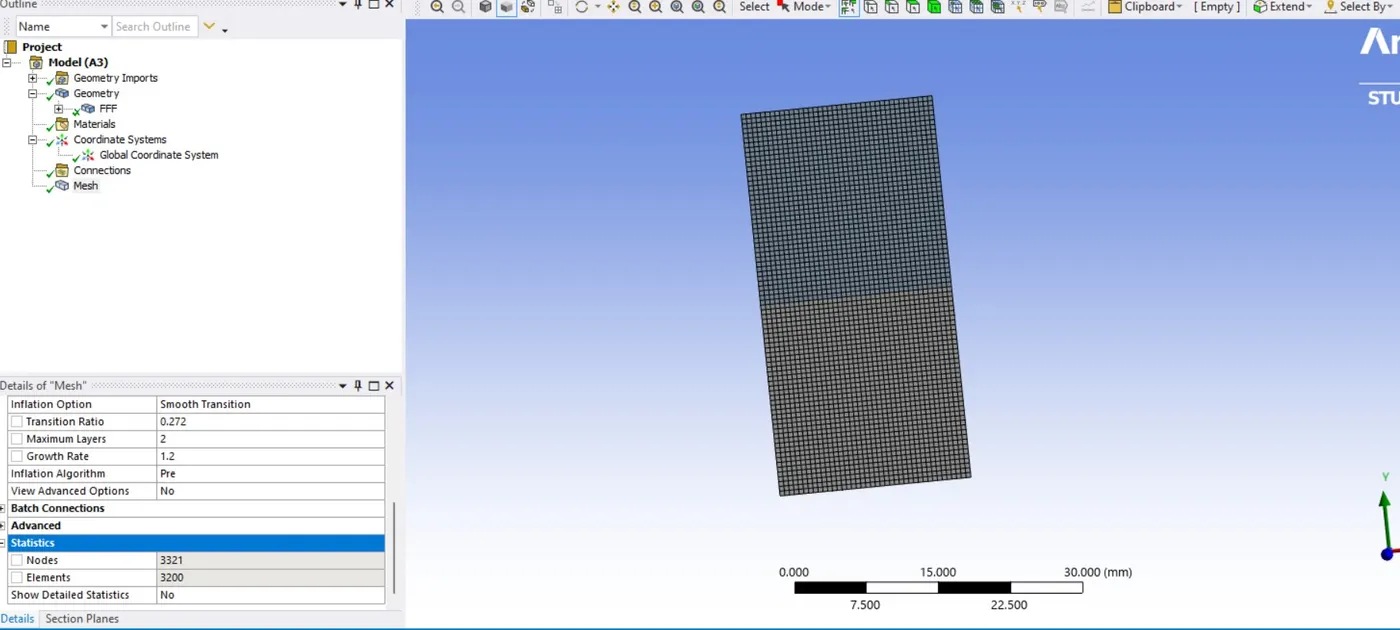
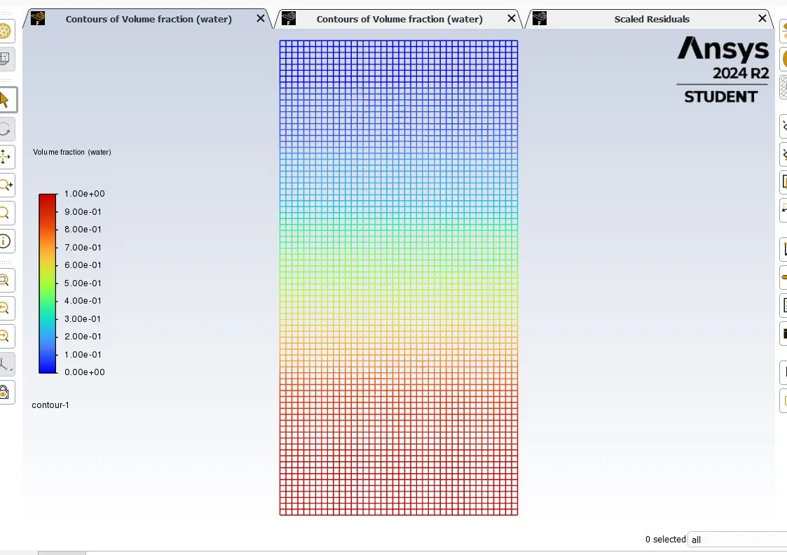
Meshing:- Open meshing section and click on the element size and set it to 0.5mm.

Now click on generate mesh and overserve the meshing.(Nodes=3321, Elements=3200)

check the number of nodes and elements and check the quality and the close the meshing.

Case-2

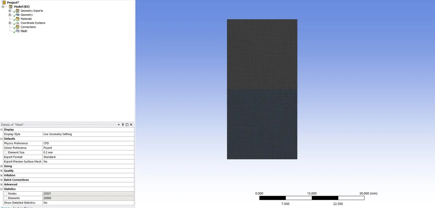
Meshing:-(Refined mesh)

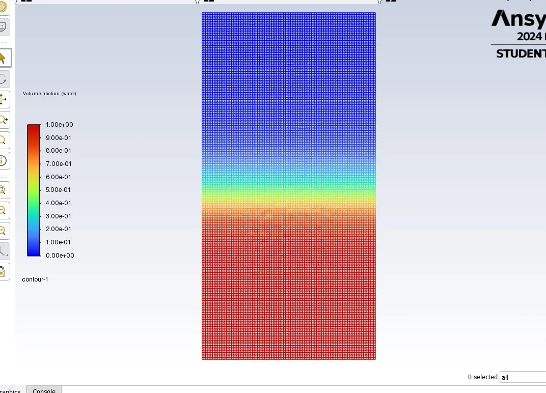
(Element size -0.2 mm) Nodes -20301, Elements-20000

Setup:-

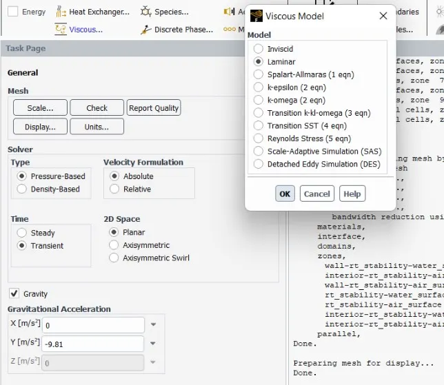
Select the pressure based solver and transient state approach.

Select gravity and give the values x=0m/s^2,y=-9.81m/s^2.

select the viscous model and select laminar model.

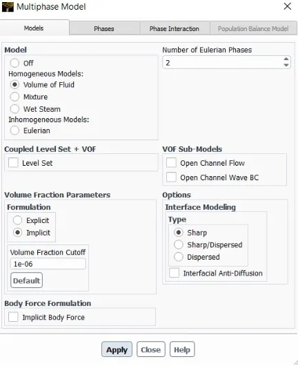
Go to multiphase model and select volume of fluid model and then set implicit formulation.

Here energy equation is not used since there is no temperature involvement.

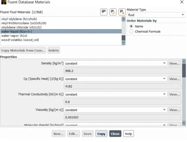
Now click on materials and add the materials, we are using 'air' and water in this simulation.

Then add water from fluent database materials.

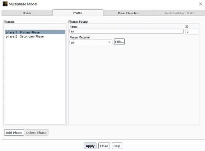
Now go to multiphase and click on phases, select air as primary phase material and water as secondary phase material.

Check the domain and see that the bottom surface is air and the upper surface is water for confirmation. Also perform mesh check.

Initialize the problem with standard initialization method since we are using transient state approach.

In the third case of the simulation we have to give a user-defined material in materials in place of air and set it to primary phase. water is to be given as second phase material as usual.

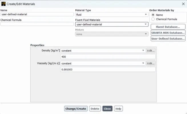
And now we go to domain and check the zones and just display and see the surfaces to remember what we have to patch.(i.e. Ansys allocates various names to the surfaces and we have to remember the water surface)

Now select standard initialization method and slick on 't =0 initialize".

Now we go to patch and for water set the volume fraction=1 for water surface (rt-stability -water-surface)and 0 for air surface.

Now under solutions- calculation activities, double click on run-calculation, select fixed type, give the number of time steps=300, Time step size=0.002

Create a contour for volume fraction for water phase.

Create a time step animation for the volume fraction of water for every two time steps.

Run the calculation( wait for sometimes to complete the calculation by Ansys, if you find any floating point error then check the meshing again and check quality criteria, aspect ratio and give better size element size and do meshing and again do the calculation.

Results:-

Scaled residual:-

case:-1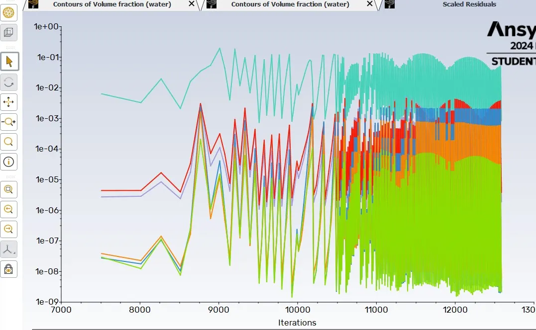

case:-2

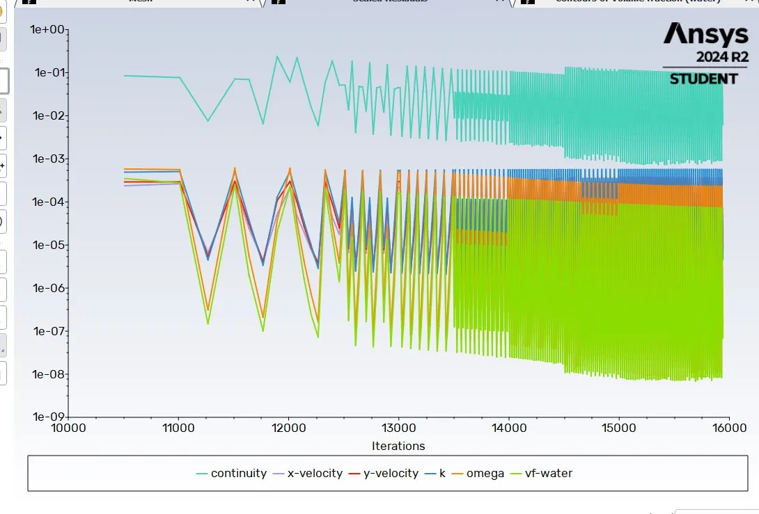
Case:-3

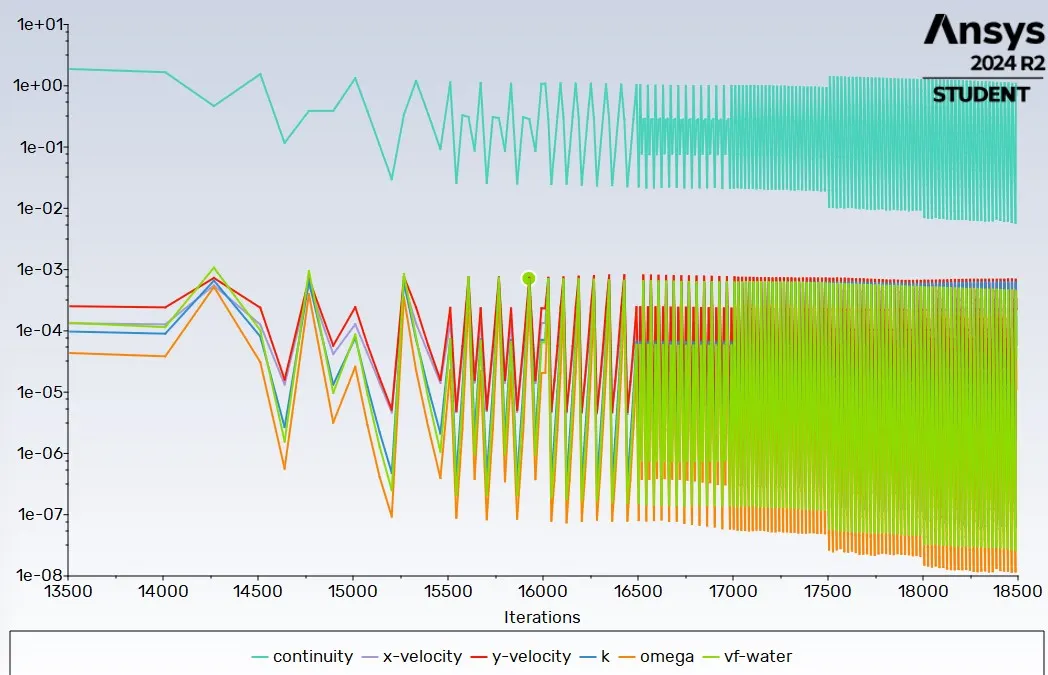
Contours of volume fraction:-

case:-1

Case:-2

Case:-3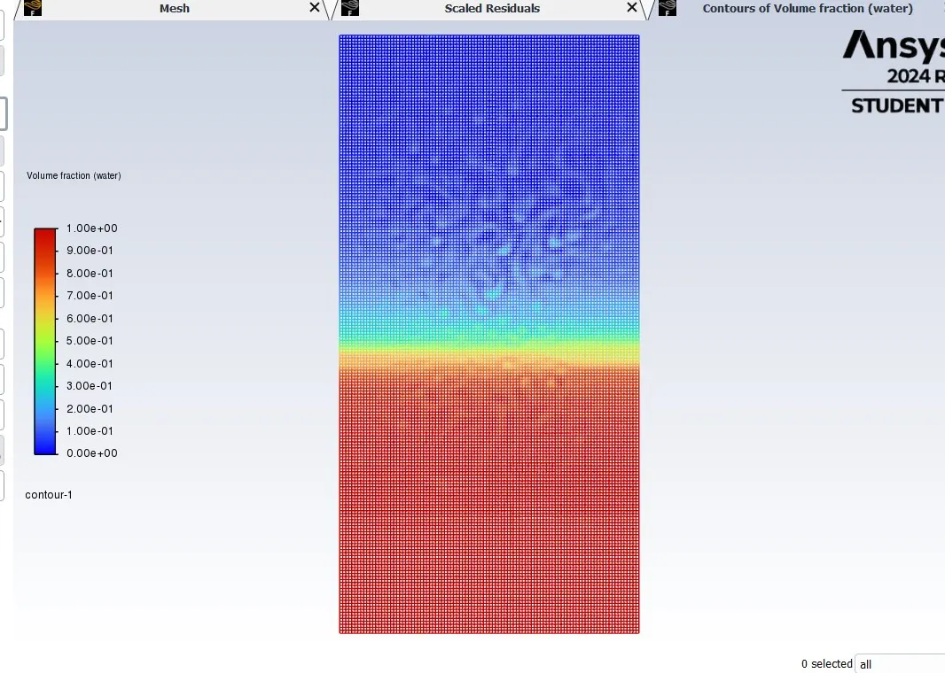

Case:-1

Rayleigh Taylor instability Animation video -0.5 mm grid (water and air)

https://drive.google.com/file/d/1jifB3EOG_-yGctWyOxQWCbf8qJ-siexx/view?usp=drive_link

Case:-2

Rayleigh Taylor instability Animation video -0.2 mm grid (water and air)

https://drive.google.com/file/d/1tV_WecvU1QrM3MzOOVV3w6VhC_aVC9kc/view?usp=drive_link

Case:-3

Rayleigh Taylor instability Animation video -0.2 mm grid (water and user defined material)

https://drive.google.com/file/d/1DKYSet2kfq8v_RxZckQGIOV9cshkmz6G/view?usp=drive_link

Atwood number:- It is a dimensionless number which is used to study hydrodynamic instabilities in density stratified flows. it is dimensionless density ratio defined as

A= (ρ1-ρ2)/ (ρ1+ρ2)

Where ρ1= Density of heavier fluid

ρ2= Density of lighter fluid

Atwood number is an important parameter in the study of Rayleigh-Taylor instability and Richtmyer-Meshkov instability. In Rayleigh Taylor instability, the penetration distance of heavy fluid bubbles into the light fluid is a function of acceleration time scale, Agt^2 where g is the gravitational acceleration and t is the time.

Calculation:-

A= (ρ1-ρ2)/ (ρ1+ρ2)

For Air -Water RT instability

ρ1=998.2kg/m3

ρ2=1.225kg/m3

A=(998.2-1.225)/(998.2+1.225)

A=0.998

For water- user defined martial RT instability

ρ1=998.2kg/m3

ρ2=400kg/m3

A=(998.2-400)/(998.2+400)

A=0.428

Behavior of the Atwood number on instability:-

Rayleigh Taylor Instability evolves in three distinct stages. Linear stability, Mushroom head falling or bubble rise formation, long term evolution due to bubble merging and mixing. for low Atwood number, bubble and mushroom head shape is relatively symmetrical. The disturbances are linear for a larger time. for large Atwood number, bubble and mushroom shapes are less symmetrical and it occurs rapidly leading to a non-linear growth rate.

Conclusion:-

The mesh with smaller element size gives the Rayleigh Taylor instability waves better than the mesh with larger element size. But it takes more time for the simulation to complete the calculation in case of finer mesh.

Finer mesh shows the formation of bubbles observed.

Compared to air, the user-defined material has more density and so it takes more time to settle down.

Since the simulation involves capturing instabilities which are changing in an unpredictable manner as function of time, transient approach is preferred over steady state approach. So the steady state approach might not be suitable for these simalations.