Week 5 - Rayleigh Taylor Instability

Aim:

1. In this challenge, we must explain some practical CFD models based on the mathematical analysis of Rayleigh Taylor waves.
2. We need to perform the Ryleigh Taylor instability simulation for 2 different mesh sizes with the baseline mesh being 0.5 mm. and then compare that result by showing the animation video. and then we need to observe the differences in the animation and also we need to explain the effect of mesh size on the simulation. [we need to choose Air and Water for this simulation].
3. We need to do one more simulation with water and user-defined material [density = 400 kg/m³, viscosity = 0.001 kg/m-s].
4. we need to explain why the steady state approach might not be suitable for this simulation type.
5. we need to define the Atwood number and also find out the Atwood number for both the cases and then we need to explain how the variation in the Atwood number in the above two cases, and how it's affecting the behavior of the instability.

Theory:-

Introduction:

• Here we are going to analyze the Rayleigh Taylor instability simulation so, that we have a dense fluid on the top and light fluid on the bottom. And that interface will be unstable when the geomentry is present here and this will result in a lot of cool-looking patterns.
• When we have two fluids like the heavier fluids, which are mixed with the lighter fluid due to the gravity and the density variations, the liquid's interface is unstable. so, the instability of the interface between the two different densities when the lighter fluid is accelerated towards the heavier fluid is known as Rayleigh-Taylor instability.
• Mainly we are doing this simulation is for to learn two things. one is we will learn something called the "volume of fluid" method. which is an important technique used to simulate two-face flow and that is why we are working on this particular problem.

Practical Applications:

1. Cavitation in boat propeller fan, when the boat propellers are turning to the right or left direction side because of the boat turning, there is a sudden non-equilibrium and fluid instability.
2. bubbles form when the water boils. so, when the water is boiling from there the bubbles are created so fluid patterns are unstable.

Reason for the steady-state approach might not be suitable for this simulation type?

Here, we use a transient (unsteady) state for this simulation and not a steady state simulation. This is because the steady-state simulation gives the final state that is reached by those fluids. so, simulating with a steady-state approach will try to solve for the final state solution of the fluid for each iteration where in the transient case, the flow is captured for each time step which gives the exact solution at the time of the simulation.

So, There is an unsettling of an interface generated with time due to the penetration of heavier fluid and lighter fluid into one another.

Explain the effect of mesh size on the simulation.

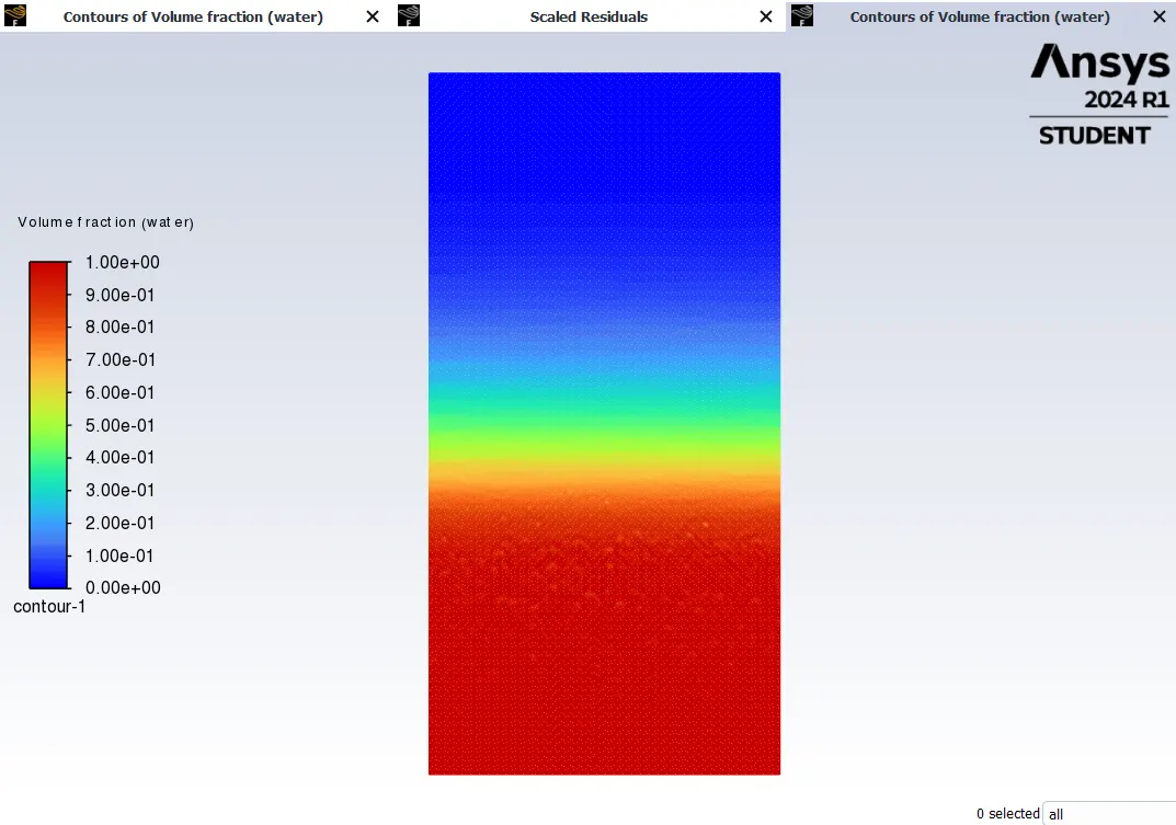
• In case 1 we have greater mesh size due to fluid mixed in the form of layers as compared with case 2 where the fluid mixed in the form of small and accurate layers which indicates the mesh size is smaller than case 1 and the density of the fluid is same for both the cases. so, these cases show clearly how the denser fluid takes place into the less denser fluid due to gravity.
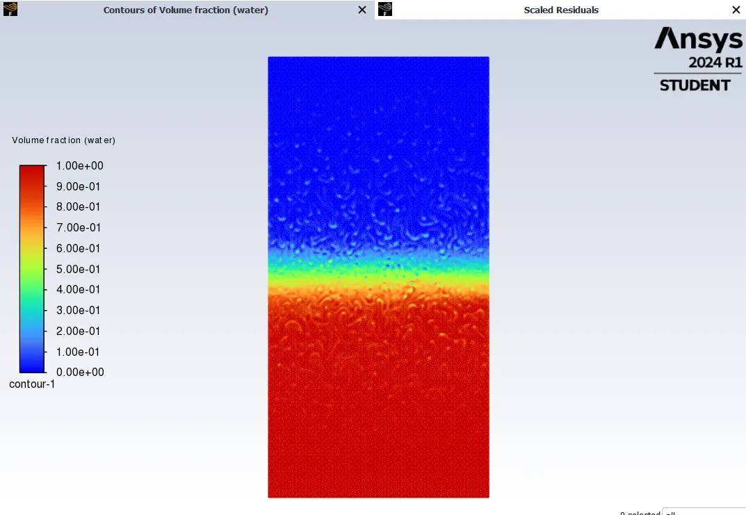
• Talking about case 3 and case 4 the mesh is more refined (0.1 mm) and both the mesh sizes are the same. In case 3 the fluid is mixed in the form of particles and the density of the fluid is the same as in cases 1 & 2. In case 4 the density of the fluid takes more time to get settled and the mesh size is the same as in case 3. So, this happened because of the density differences between the two cases 3 & 4. In case 3 the density difference was high and the density difference was low in case 4.
• so in this experiment the time taken is more because of the smaller and finer mesh size used. Also, the densities of the two fluids are different. Finally, the effect of changing the mesh size takes more time to simulate and we get accurate results out of it.

Practical CFD Model that is based on mathematical analysis of Rayleigh Taylor waves:

• Rayleigh Taylor instability:

The Rayleigh Taylor instability is an instability of an interface between the two fluids of different densities which occurs when the lighter fluid is pushing the heavier fluid. When the fluids are accelerated means, the less denser fluid accelerates into the denser fluid. This occurs deep underwater on the surface of an expanding bubble and in a nuclear explosion.

The RT instability develops from the initial perturbations progress from a linear growth phase into a non-linear growth phase, eventually developing the "plumes" flowing upwards. and "spikes" falling downwards. The differences between the fluid densities divided by their sum are defined as the Atwood number(A). if the A close to 0 means RTI flow takes from the symmetric "finger" of fluid. for A close to 1 means the much lighter fluid is below the heavier fluid and takes the form of large bubbles like plumes. so, the instability of the interface between the two different densities when the lighter fluid is accelerated towards the heavier fluid is known as Rayleigh-Taylor instability.

• Saffman-Taylor instability:

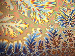
The Saffman-Taylor instability is also known as viscous fingering. it is the formation of a pattern in a morphologically unstable interface between two fluids in a porous medium. This method is most often encountered during drainage processes through media such as soils. It occurs when the less viscous fluid is injected and displaces a more viscous fluid. If this is in the inverse situation, with the more viscous fluid displacing above the other. so, here there is no instability seen.

Essentially the same effect occurs driven by gravity (without injection) if the interface is horizontal and it separates the two fluids of different densities the heavier fluid is above the other so, this is called Rayleigh Taylor's instability.

• Richtmeyer Meshkow instability:

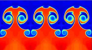
This occurs when the two fluids of different densities are impulsively accelerated. But normally this happens by the passing of a shock wave. The development of instability begins with small amplitude perturbations which initially grow linearly with time. But this is followed by a nonlinear regime with a bubble appearing when in the case of a lighter fluid penetrating a heavier fluid, and with spikes appearing when in the case of a heavier fluid penetrating a lighter fluid.

The chaotic regime eventually reached and the two fluids mixed. This instability can be considered the impulsive acceleration limit of the Rayleigh Taylor instability.

• Plateau Rayleigh instability:

In fluid dynamics, the Plateau Rayleigh instability is just often called Rayleigh instability. To explain why and how a falling stream of fluids breaks up into smaller packets with the same volume but less surface area. so, It is related to Rayleigh Taylor's instability and is part of a greater branch of fluid dynamics concerned with fluid thread breakup. This fluid instability is exploited in the design of a particular type of inkjet technology whereby a jet of liquid is perturbed into a steady stream of droplets.

The driving force of the Plateau Rayleigh instability is that liquids, under the same tensions, tend to minimize the surface area.

• Kelvin Helmholtz instability:

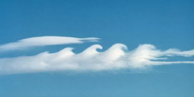
The Kelvin Helmholtz instability is a fluid instability that occurs when there is a velocity shear in a single continuous fluid or a velocity difference between two fluids. The Kelvin Helmholtz instability is visible in the atmosphere of planets and moons, such as cloud formation on Earth or the red spot on Jupiter, and the atmosphere of the sun and other stars as well.

Courant Number:

The Courant number is a dimensionless number named after the mathematician Richard Courant. The Courant number is used in CFD simulations to evaluate the time steps requirement for transient simulations for a given mesh size and flow velocity. It is linked to the Courant-Friedrichs-Lewy(CFL) stability conditions of numerical schemes.

C = UΔt/Δh

Where,

• U - Flow velocity.
• Δt - It represents the time step of the simulation.
• Δh - The characteristic size of the mesh cell. (i dimension)

For, multi-dimensional problems the condition can be evaluated as the sum in all directions, i.e

C = ∑_i (U_iΔt / Δh_i)

In CFD simulation, The courant number broadly indicates how much the information travels (u) across a computational gird cell (Δh) in a unit of time (Δt). If the courant number is > 1, then it means that the information propagates through more than one cell at each time step, making the solution inaccurate and potentially leading to a non-physical result.

The Courant number plays an important role when running transient flow simulations, where we are interested in the variations of the flow field in time and as well as in space. In the CFL conditions mean stability requirements first. from the numerical viewpoint, the time integration scheme can be broadly divided into three categories they are Explicite, Implicite, and semi-implicit.

For, Explicit the scheme the solution at the time step n+1 is calculated using the known values of the solution at time n. For, Implicite the scheme the solution at the time step n+1 is calculated using the known values of the solution at time n+1. For, the Semi-implicit scheme uses both the solution at time n and n+1.

Differents between Implicit and Explicit methods:

• In this Implicit method, the unknown values are solved by using existing and unknown values from the neighboring cell. In this method, the equations are solved simultaneously. It doesn't have been a strict CFL criteria. The default value of the courant number is 5. This method is suitable for Hypersonic flow and shock interaction.
• In this Explicit method, the unknown values are solved by using the existing value from the neighboring cell. In this method, the equations are not solved simultaneously. This method has strict CFL criteria. The default value of the courant number is 2. This method is suitable for the flow having a high Mach number.

Atwood numbers:

Atwood number is a dimensionless number which is defined as the ratio of the difference between the heavier fluid density and lighter fluid density to their sum. It is used in the study of hydrodynamic instability in density-stratified flows. Atwood number is an important parameter in the study of Ryleigh Taylor instability and Richtmeyer meshkow instability.

In RTI Penetration density of heavy fluid bubbles into the lighter fluid is a function of the acceleration time scale, where g is the gravitation acceleration and t is the time. So, In this simulation when the fluids are getting started to an unstable state. The initial mixture of instability shapes is called plumes and it's basically used to analyze the plumes size and shift from plumes to eddies. The Atwood number is used to find those two things.

• Atwood number (A) = (ρ1-ρ2) / (ρ1+ρ2)

Where,

• ρ1 - Density of the heavier fluid.
• ρ2 - Density of the lighter fluid.

Calculation of Atwood number:

1. For air and water,

Here, water is the heavier dense fluid compared to air. so we take

Density of Water (ρ1), ρ1 = 998.2 Kg/m³

Density of air(ρ2), ρ2 = 1.225 Kg/m³

We know that,

• Atwood number (A) = (ρ1-ρ2) / (ρ1+ρ2)

A = (998.2-1.225) / (998.2+1.225)

A = 0.9975

2. For water and user-defined fluid,

Density of Water (ρ1), ρ1 = 998.2 Kg/m³

Density of user-defined fluid (ρ2), ρ2 = 400 Kg/m³

We know that,

• Atwood number (A) = (ρ1-ρ2) / (ρ1+ρ2)

A = (998.2-400) / (998.2+400)

A = 0.4278

Procedure:-

Geomentry (pre-processing):

• Here we will analyze the Ryleigh Taylor instability simulation so, we have a dense fluid on the top and light fluid on the bottom. And that interface is going to be unstable when geomentry I present and this is going to result in a lot of cool-looking patterns.
• Mainly we are doing this simulation is for to learn two things. one is we will learn something called the "volume of fluid" method. which is an important technique used to simulate two-face flow. and that is why we are working on this particular problem.

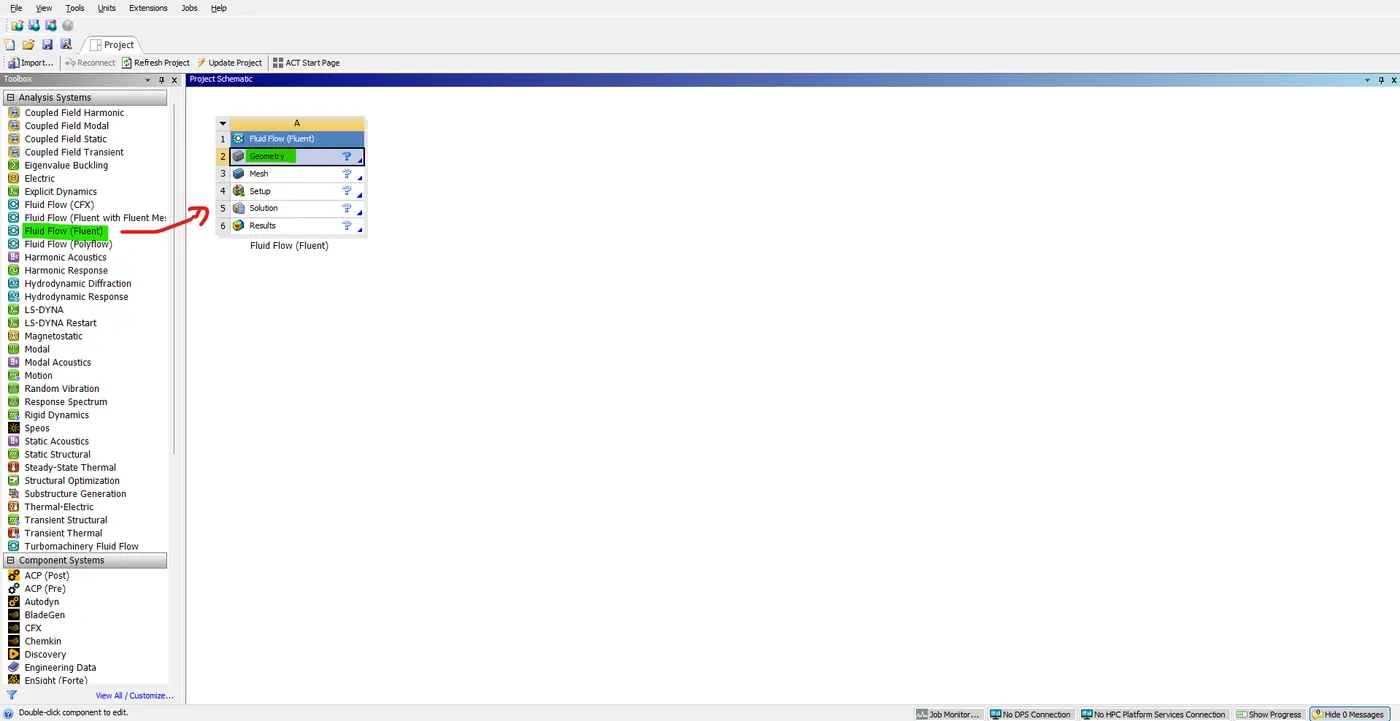
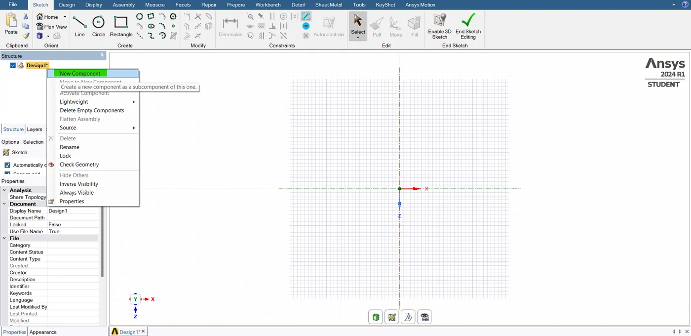
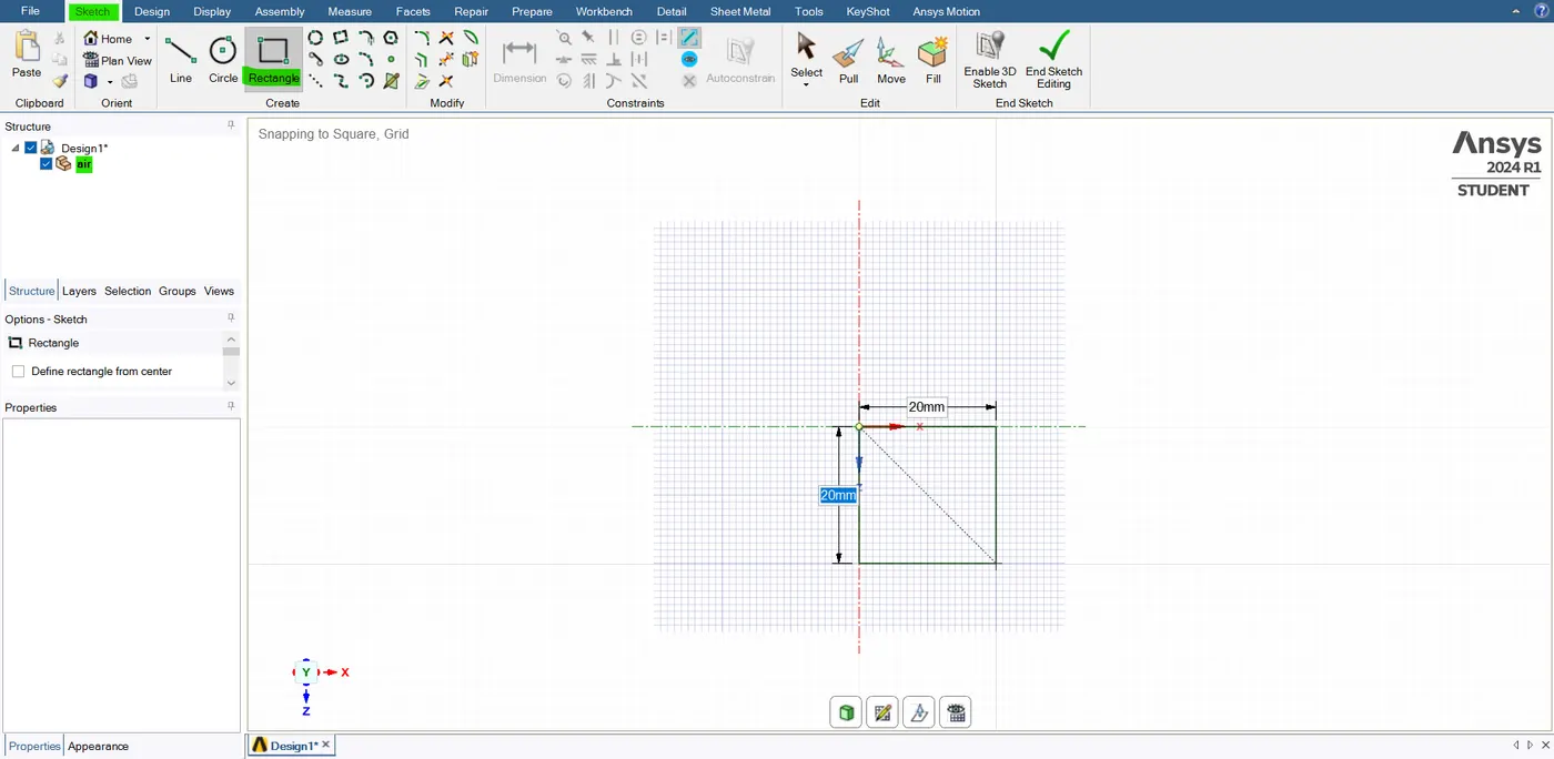
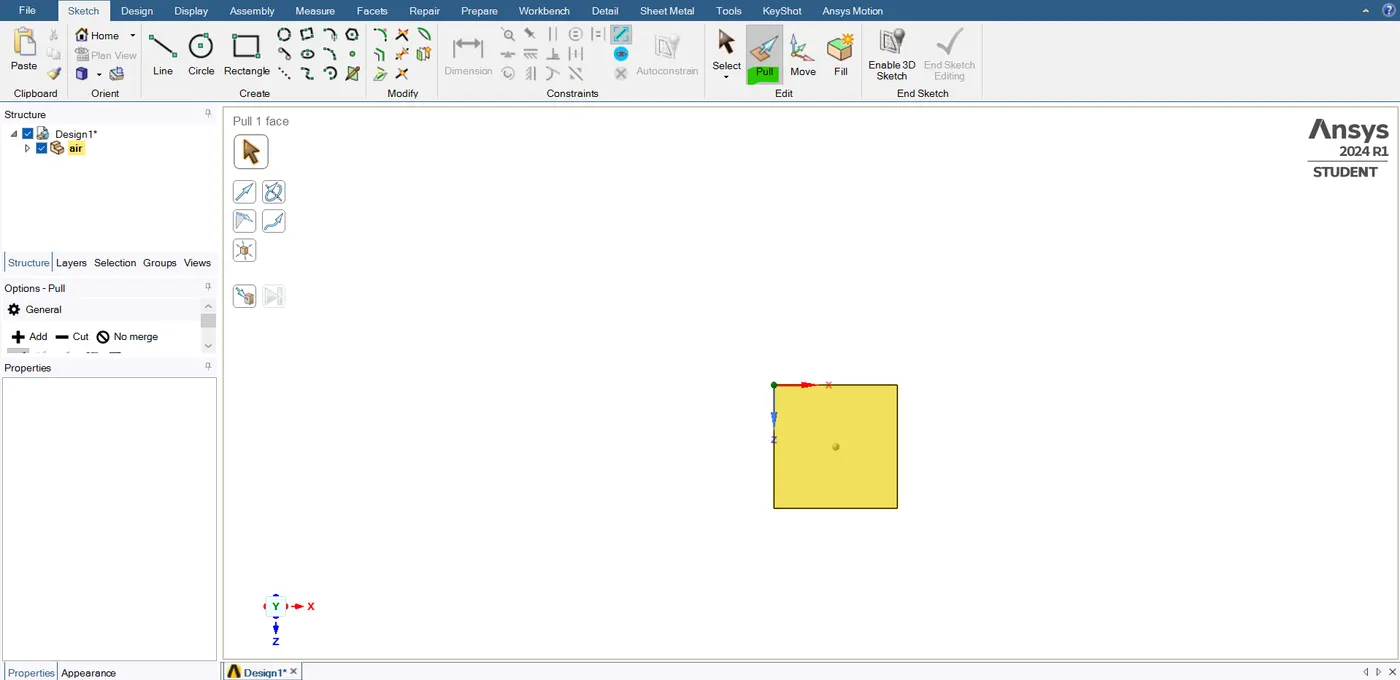
• Now this analysis is going to be in 2D. so, first thing I'm going to create a square, and the dimensions are 20 mm by 20 mm. After that, I'm going to use a pull tool to create a surface out of this. now the surface is created once I have a surface I'm going to move it to a new component called air.

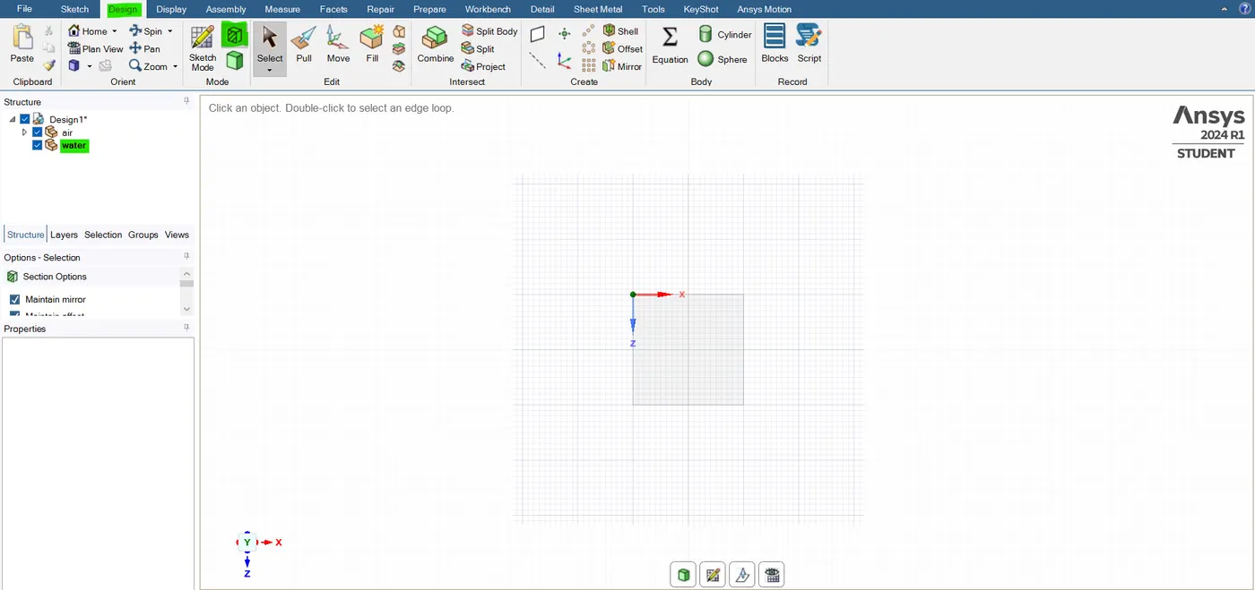
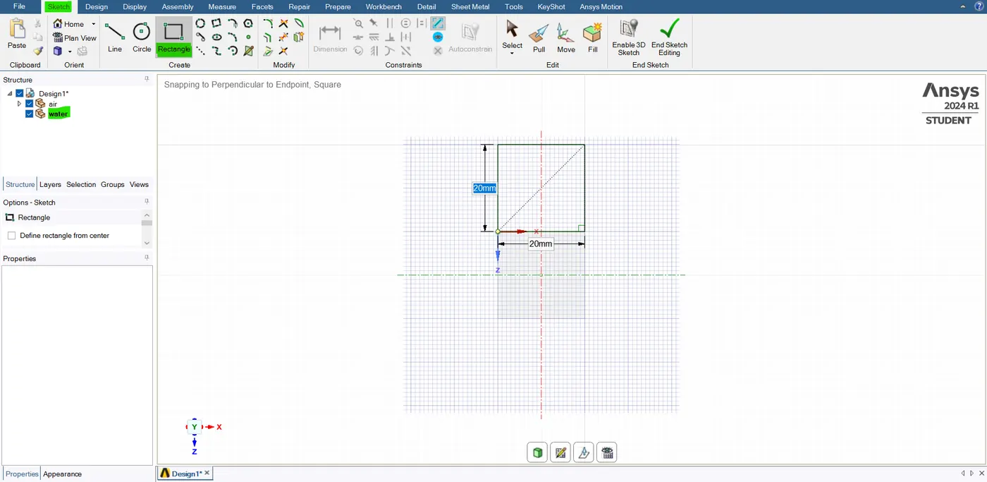
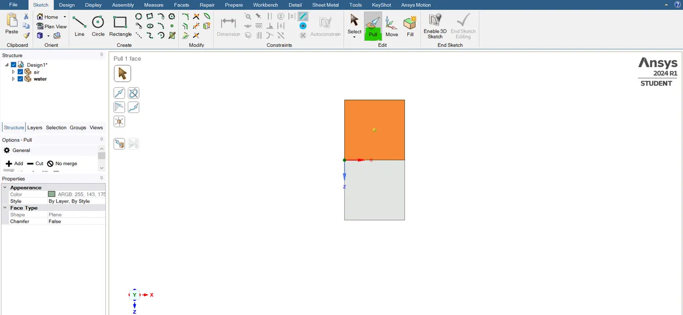
• now next thing I'm going to create a new component and it is just called water. these two components and into a "Design Domain". so that's fine. now for water, I'm going to create a new sketch. In this particular plane, I'm going to select "rectangle tool" and Then draw another square on the air component. and the dimension of water is 20 mm by 20 mm. After the use of the "pull tool". to create a surface on the air surface.

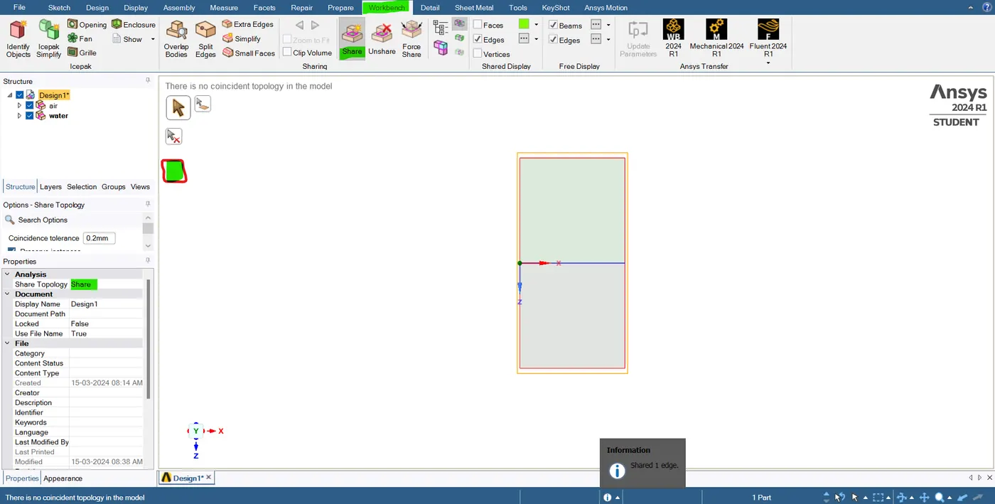
• So, now the surface has been generated. So, hit "ESC". now we have air and water. the next thing that we want to create a conformal mesh. to do that we need to enable the surfaces to share the data. so, I'm going to the workbench and I'm going to use the share tool.
• Now I'm just going to select both these components first and then I'm going to click on share. so, now you can see that one edge has been shared and the icons in the subdomain are also modified to indicate that they have been shared. and the shared topology is enabled automatically. It's set to share. so, with this close the geomentry and then open the meshing part.

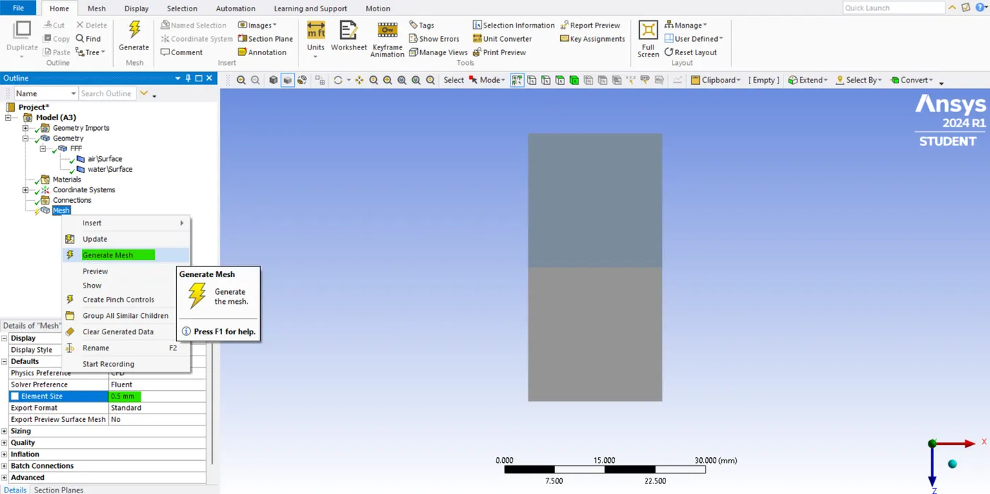
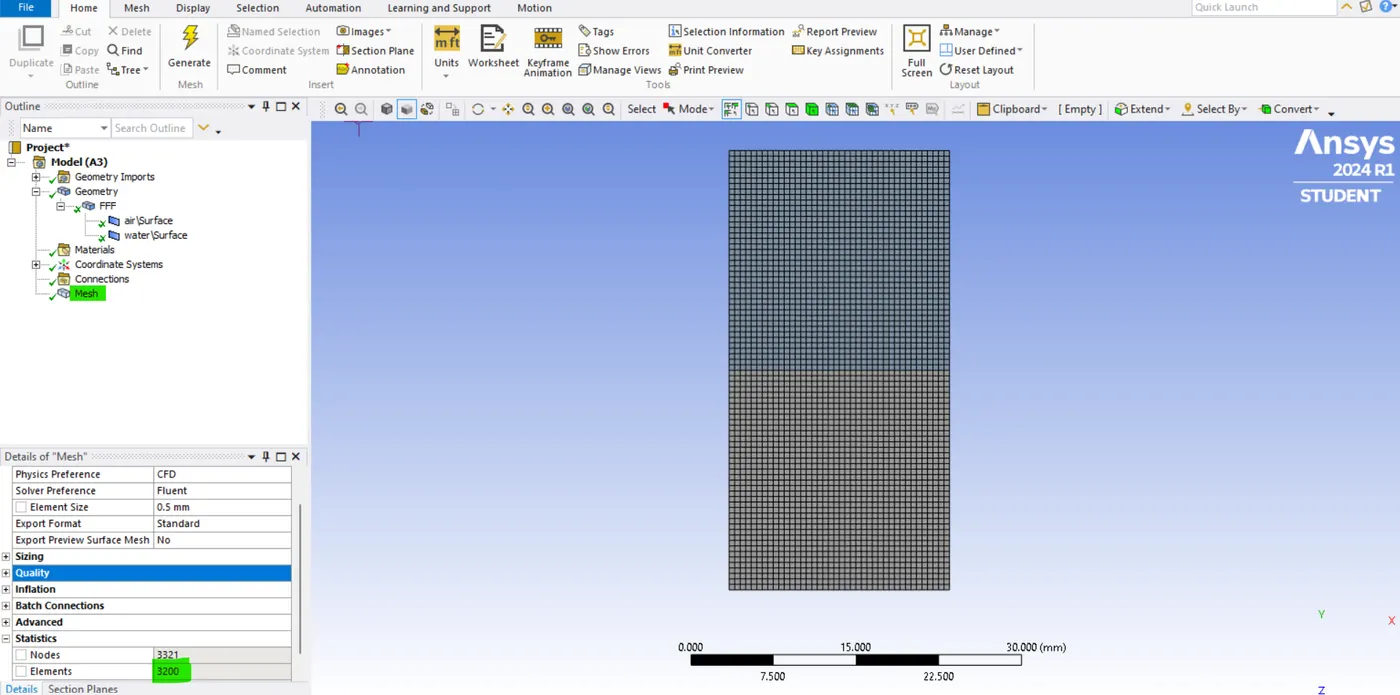
• So, the next thing is meshing. so, open the meshing part, and first, just we are going to right-click on mesh and click generate. so we are going to see first what the basic mesh looks like. now the basic mesh element is 2.3 mm. so, we need a smaller mesh something like less than 0.5 mm, and then update the mesh.

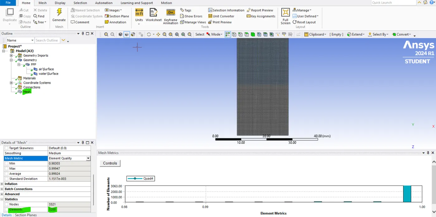
• so, this is not too fine for this simulation but this should help us to do the case "setup" and then get the initial answer first.

Setup and modeling approach:

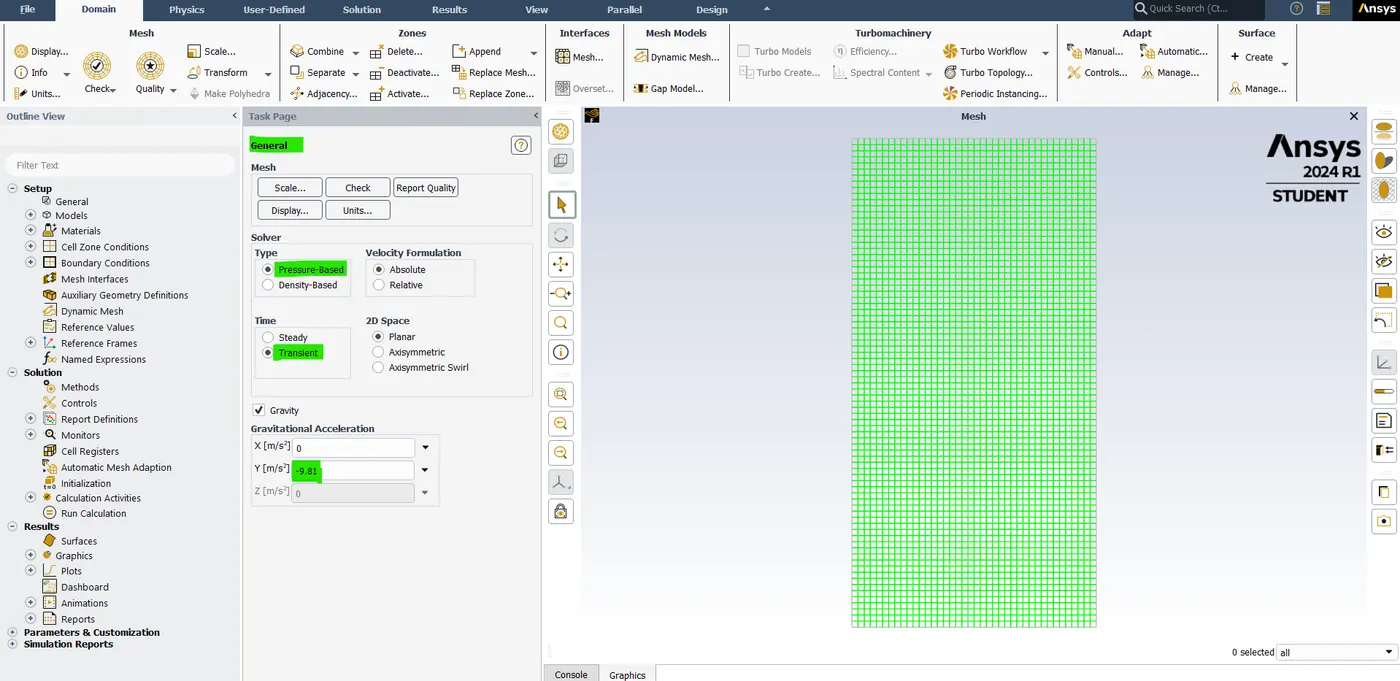
• so, the next thing is to launch the Ansys Fluent. Open the setup GUI. And so, now you can see that this is a 2-dimensional simulation and under this really on classification in the region definition but that's fine.
• so, we are interested in transient simulation because we want to see how these two interfaces collapse as a function of time. so it's very important to do this we need Gravity enabled. so, in a 2D simulation, this direction is the y-axis. so want the gravity to be in a negative direction. so, the y-axis is -9.81. so, this is going to be the value for gravity.

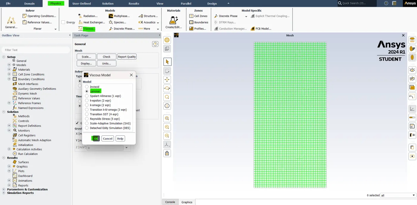
• now go to the setting up physics we don't need the energy equation and I'm going to run this in the "Laminar model". so, let's see first what happened. because the velocity should be fairly slow. so this is fine.

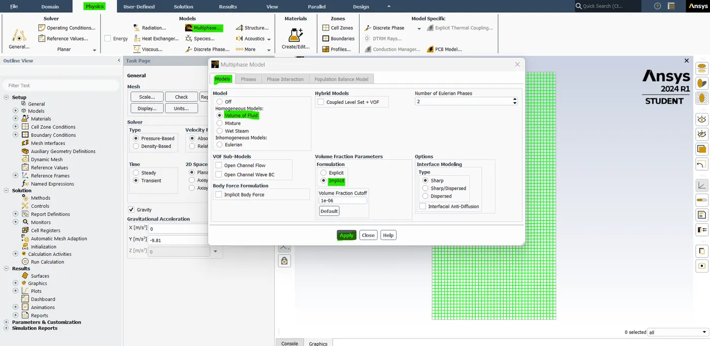
• An important step is enabling the "Multi face" model. We are interested in doing something called the "volume of fluid" method. where we have two oils in a phase that can represent the water or vice versa.
• so, here we are going to do the "implicit" formulation. and the "courant number" is set to 0.25. so, this is our stability criteria so, click"ok".

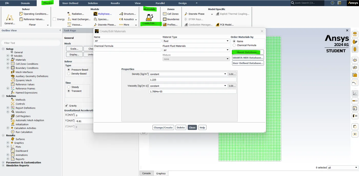
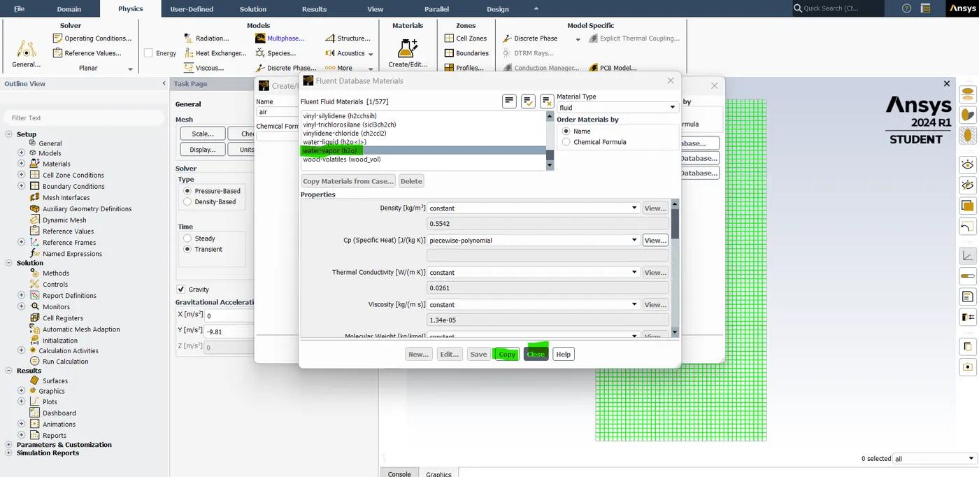
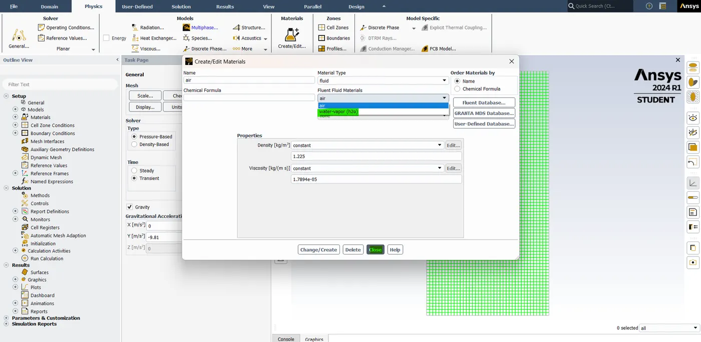
• Now go to the created material. and then go to the fluent database and then select "Water-liquid h201" and copy the material and close. so, now the water material is added to the fluid. so, close to this material properties.

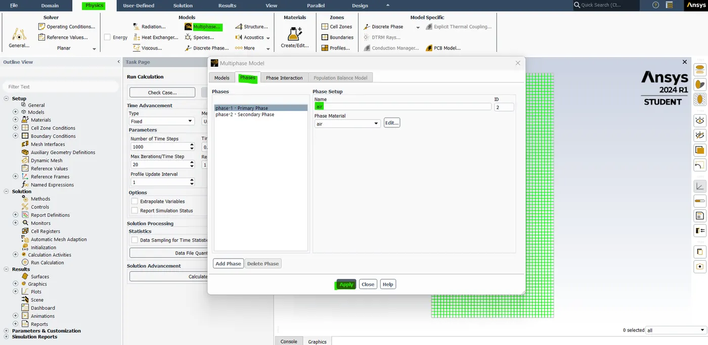
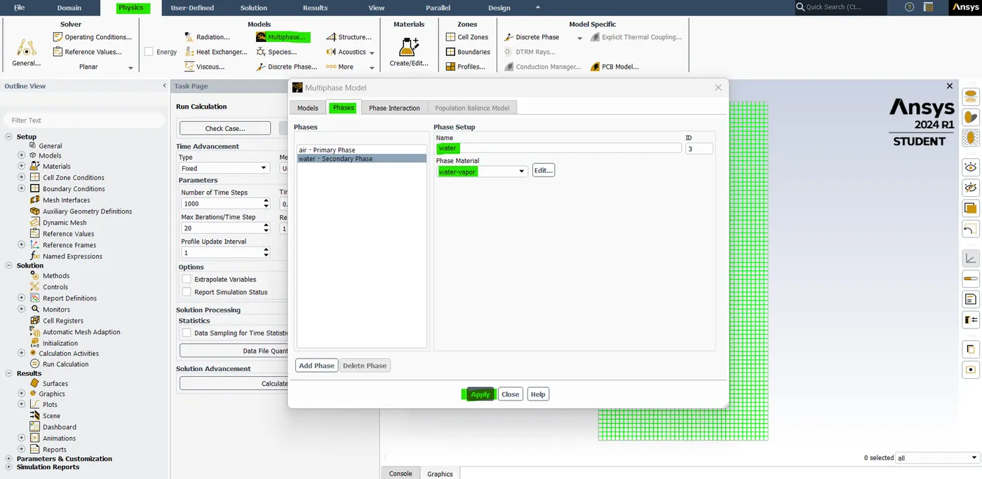
• And then now we need to "list all our faces". so our primary phase 1 name is air. And the material is air. similarly, our phase 2 name is water and the material is water. so, named "Water". so, click "ok".

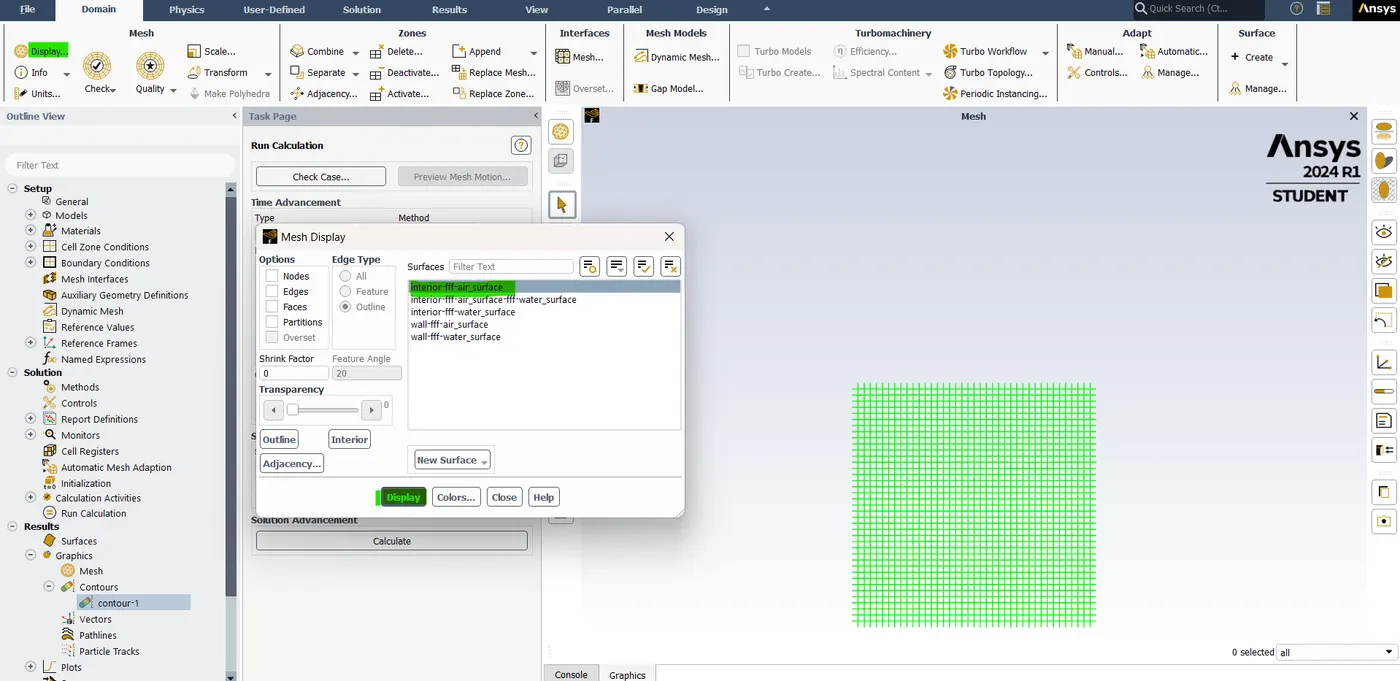
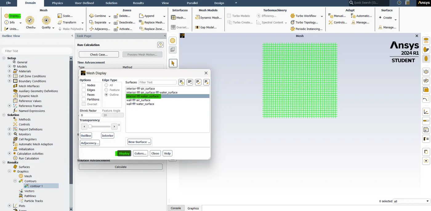
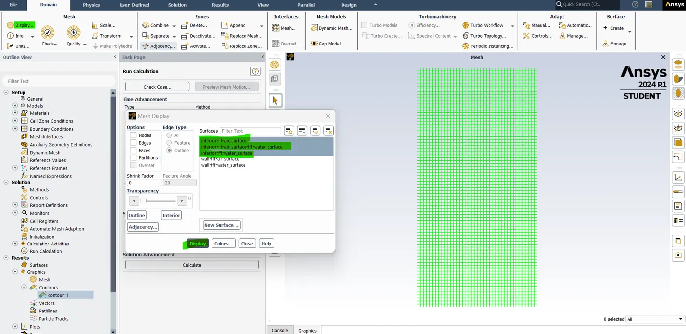
• Now go to setting up the domain and then click display. so, we want to check out the Zones here. so, I'm just going to look at one surface at a time. so this basically should be our "air" because this is in the Bottom. Similarly, this needs to be the "water" because this is at the top. The reason why it's important to remember is that we are going to do something called a "patch".

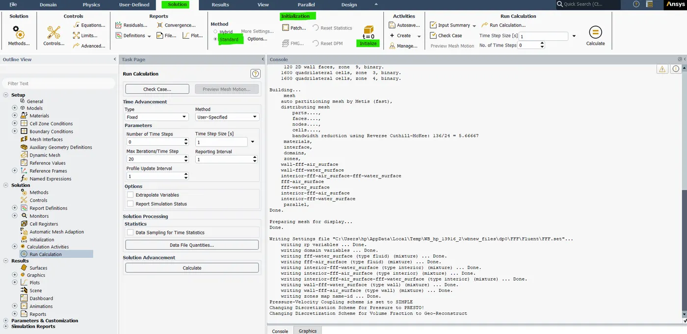
• To do that let's go to the "solving" section. And then first do the standard initialization. when we do this nothing happens because there is no inlet flow and outlet flow.

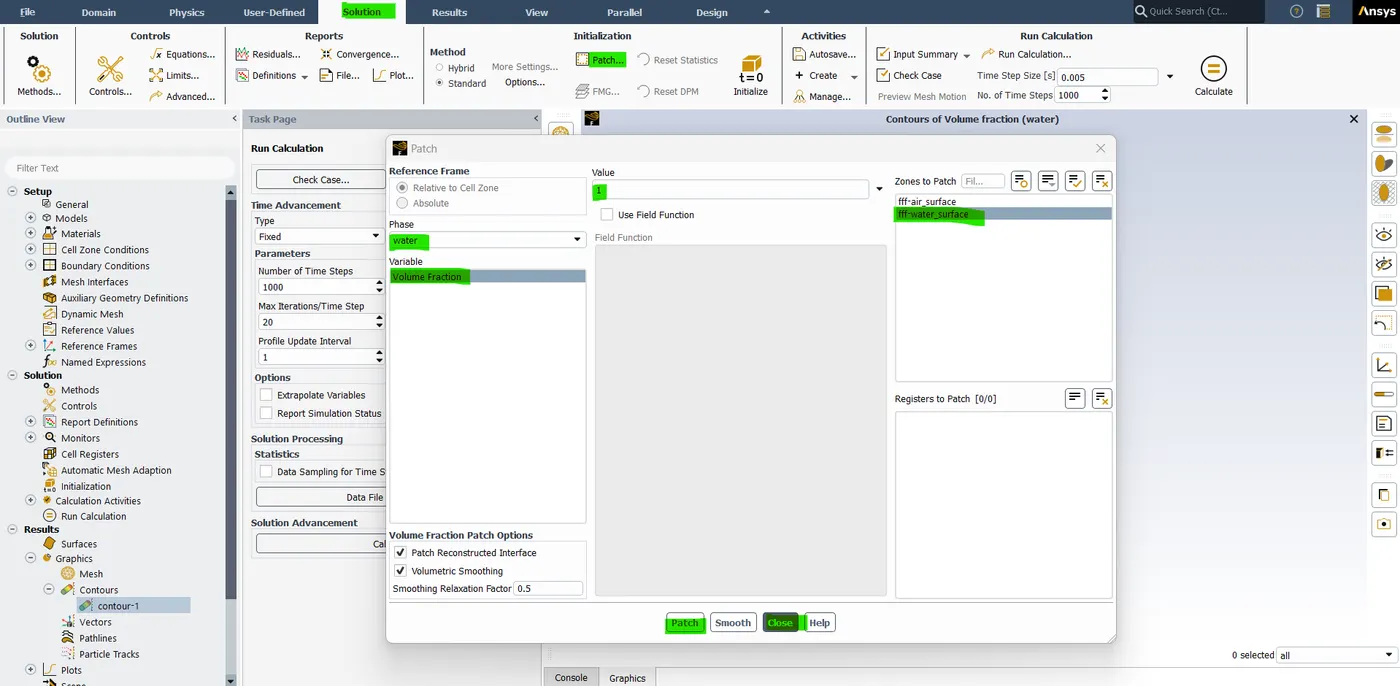
• Now you can see this option called "patch". now in this patch, I'm going to select a "water" phase and "volume fraction" in the select variable, and in the zones select the water surfaces. enter the value is 1 and then hit patch it.

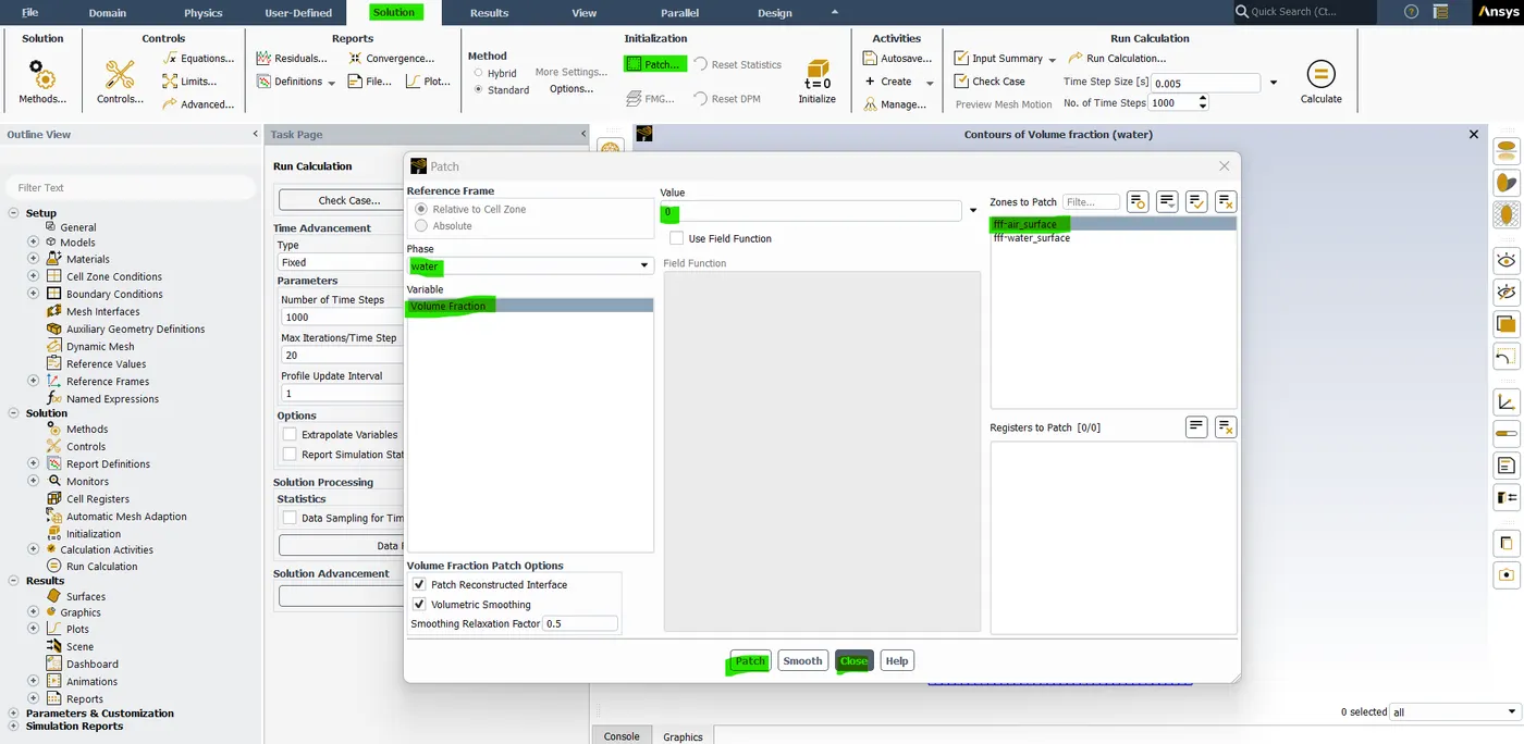
• Similarly, select the air in the zones and then enter the value is 0. and then hit patch it. so, what does this value mean? when we are driving two faces these faces are represented by a value called "Alpha". If alpha is "1". it represents one face, it could be water or air. And similarly when the Alpha is "0". it represents the other phases.
• So, for example, Let's say that when alpha equals = 1, we have water. it means when we initialize we want the Alpha to be "1" at the top and the alpha to be "0". at the bottom. so, this means that your initialization process is correct and this is very important.

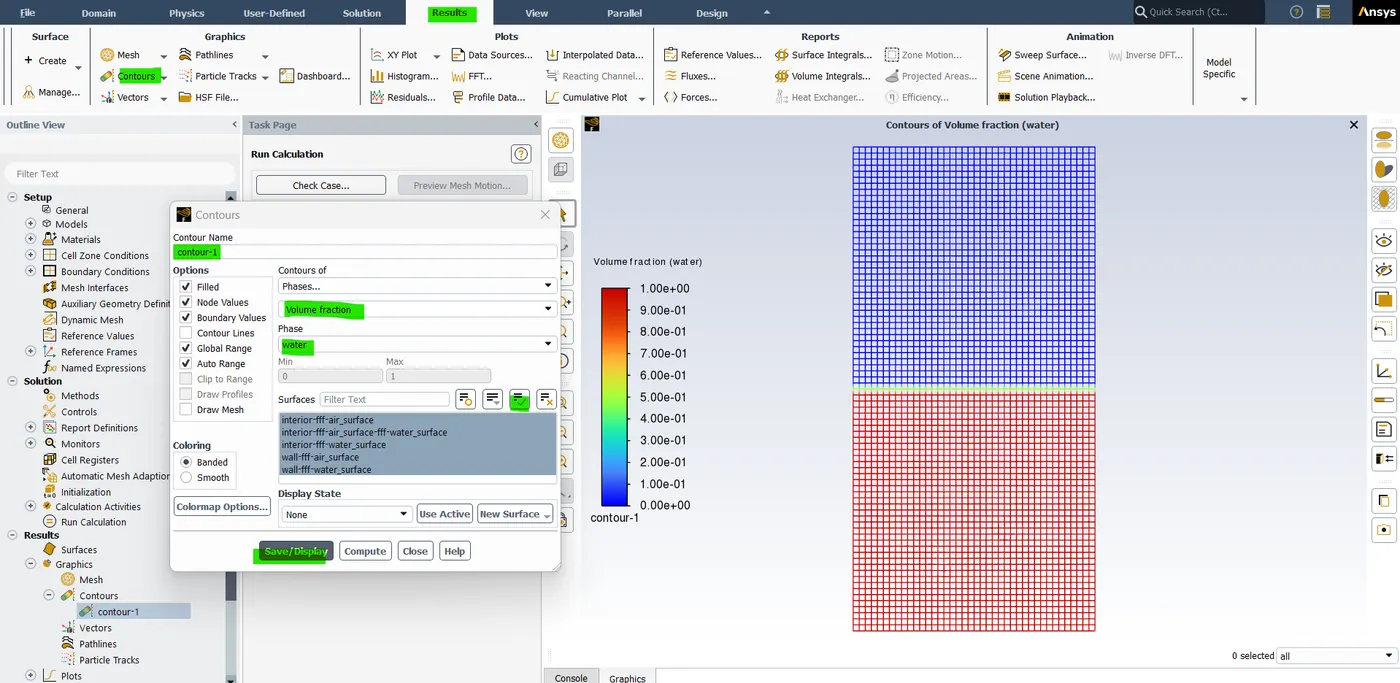
• so, now how do we make sure that the initialization was set correctly? so, to verify that we need to go to post-processing and create a new "contour plot" on "phases". select the phase as water, select all surfaces, and click "ok".

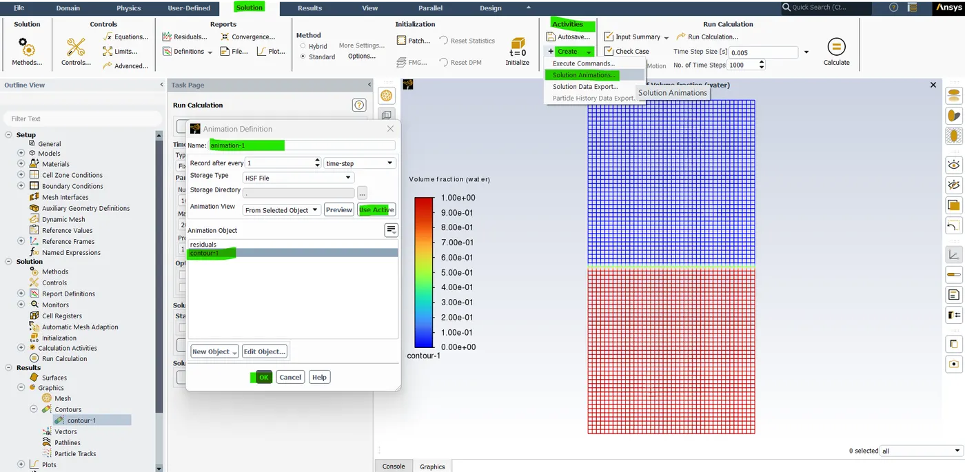
• The other thing that we need to do is we want to create the "solution animation" of our contour and I want to do it every time steps right.

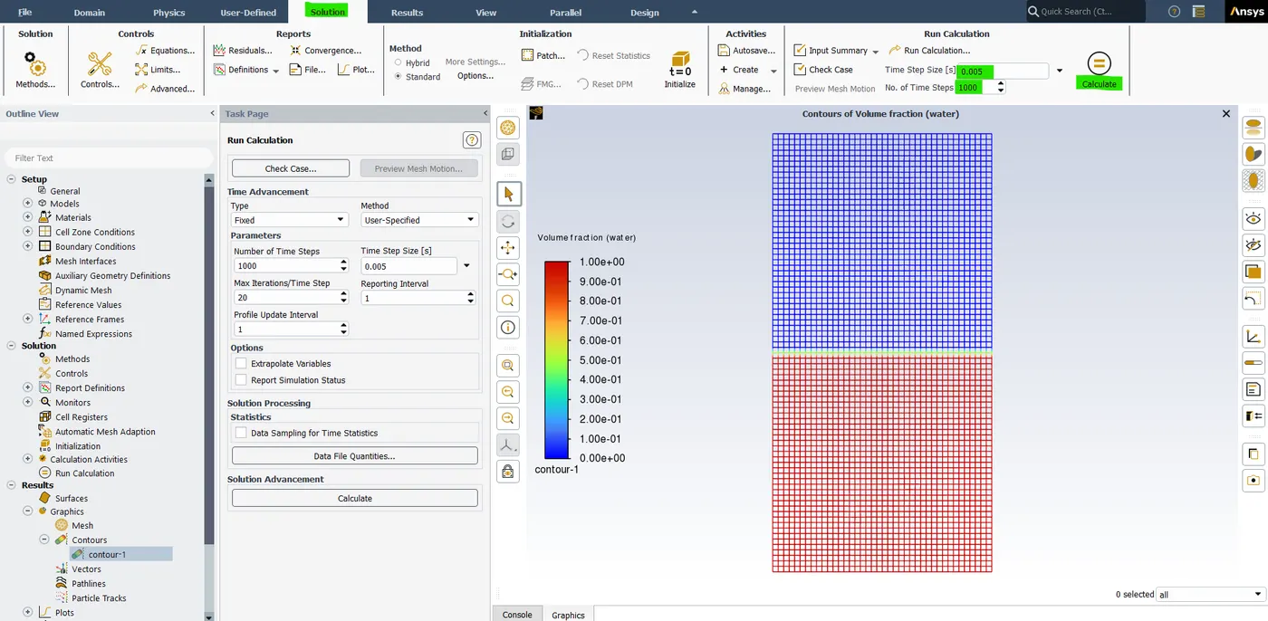
• So, when we do that the volume fraction of water is "1" at the top and it's "0" at the bottom. so, it tells me that the setup is perfect. now let's go to the "solving" section and in the "Run calculation" as far as the time step is concerned I'm going to pick a very reasonable value. so, I'm going to start with the value of 0. and I want to run 0.005 iterations. so we need to run 1000 time steps to see what happens. and we are going to use the "fixed time step" method.
• If we have a smaller time step size the computational time will be more but it will give good results. similarly, if we have a bigger time step size the computational time will be more and it will get a void exception error which means due to the higher time step size it won't be able to capture the fluid motion in every element.
• It also depends on the mesh if we have a mesh size of 0.1mm and we are using the time step size as 0.001 m/s then it will create a void exception error so, we won't get the solution.
• Although deciding the time step size is hit and trial method we should start with a smaller time step and then we can increase the time step size gradually.
• we can do this by giving the first 500 time steps with a smaller time step size after that increase the time step gradually.
• To find the simulation time is a product of the Time step size and no.of.time.step means, Simulation time = Time step size * no.of.time.steps.
• For the first case the Simulation time =0.005 * 1000 = 5 secs. This is just an assumption we can further more number of time steps if the solution is not done.

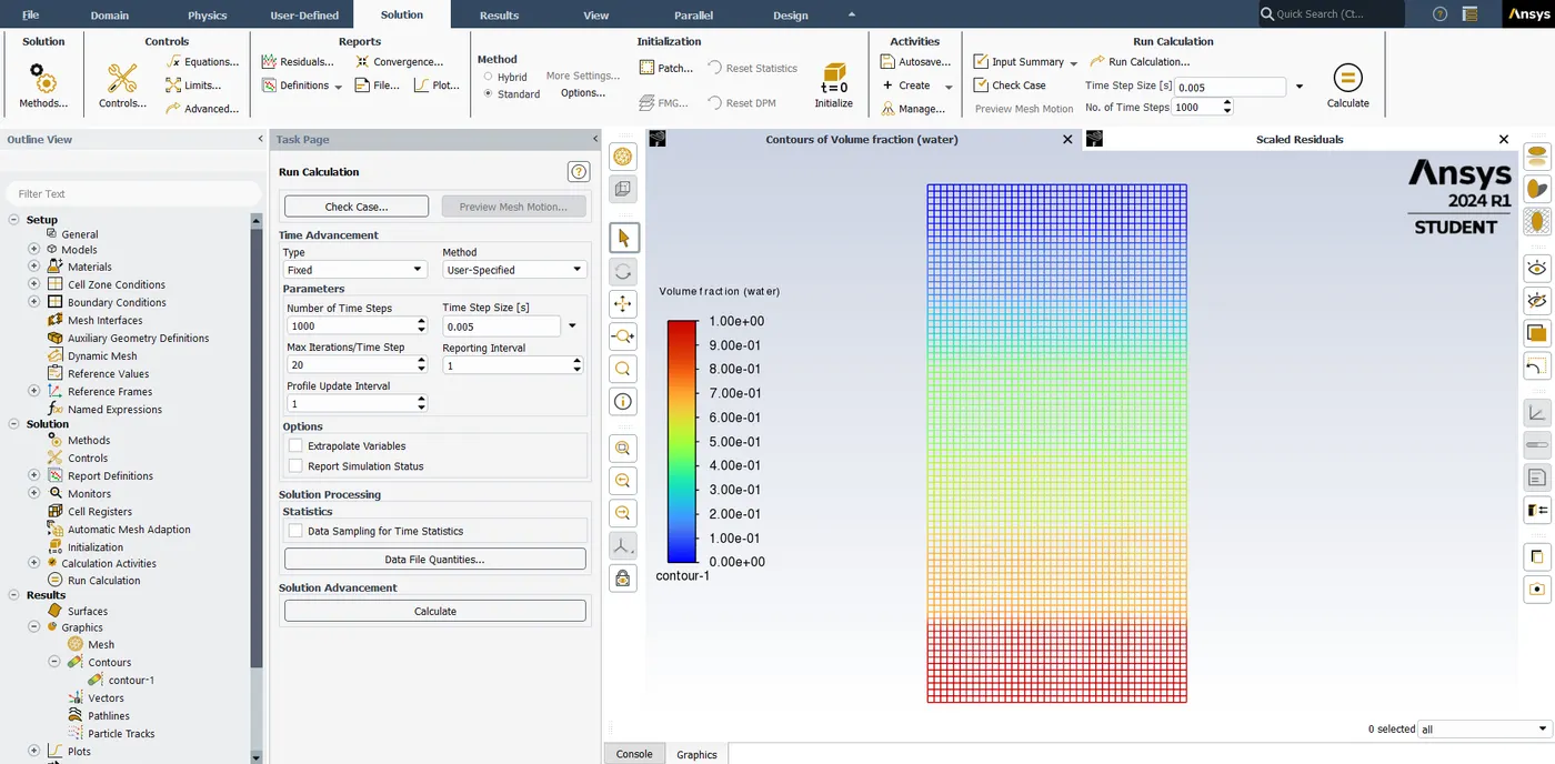
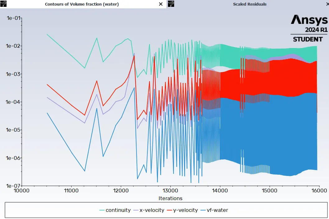
• So, click "ok" and hit "calculate". so, now you can see that the interface is getting deformed and we can see the instability. And in the console, you can see that my solution has started diverging. so, this pattern is going to be changed if our mesh computational is more and more refined and this looks quite interesting and quite beautiful to watch.

Result (post-processing):

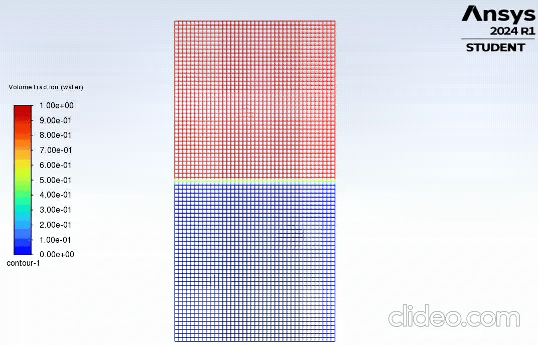
Case-1 Baseline mesh: 0.5 mm

No.of Node = 3321, No.of Element = 3200.

Contour plots:- Volume of fraction (water)

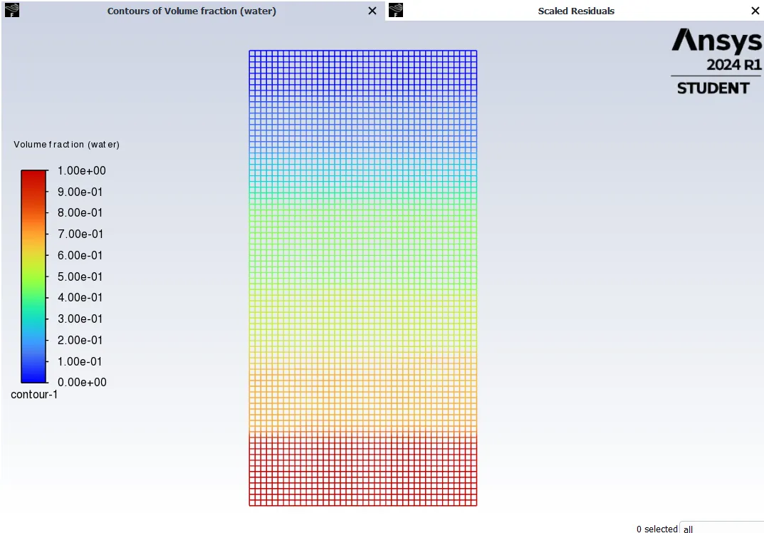
Scaled residuals:

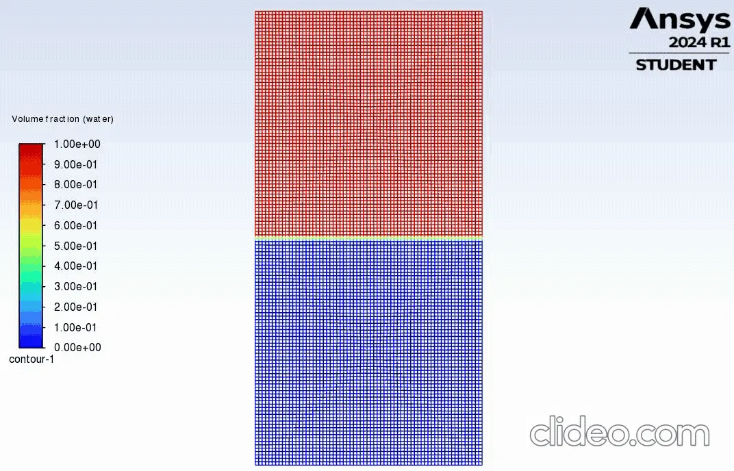
Case-2 Baseline mesh: 0.3 mm

No.of Node = 9180, No.of Element = 8978.

Contour plots:- Volume of fraction (water)

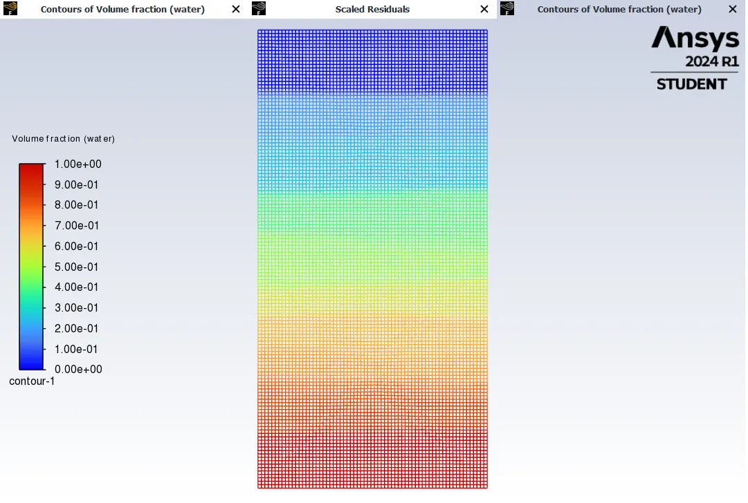
Scaled residuals:

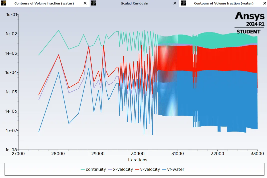
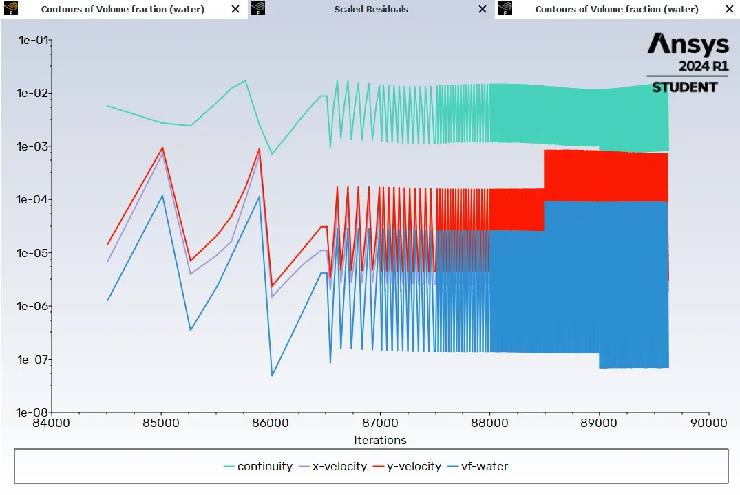
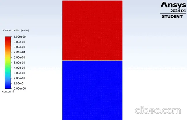
Case-3 Baseline mesh: 0.1 mm

No.of Node = 80601, No.of Element = 80000.

Contour plots:- Volume of fraction (water)

Scaled residuals:

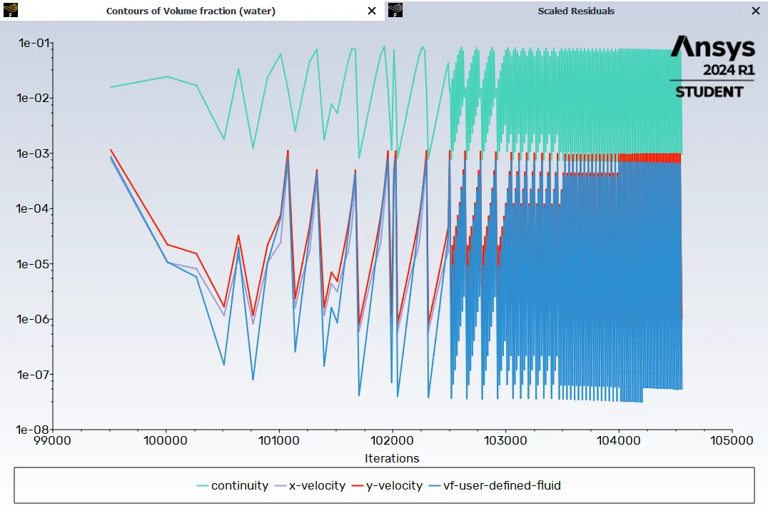
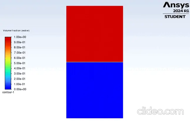
Case-4 Baseline mesh: 0.1 mm, (density = 400 kg/m3, viscosity = 0.001 kg/m-s).

No.of Node = 80601, No.of Element = 80000.

Contour plots:- Volume of fraction (water)

Scaled residuals:

Animation video file:

Case-1:

Case-2:

Case-3:

Case-4:

Grid independency test:

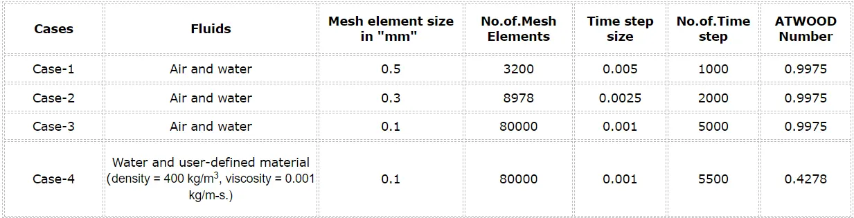
Conclusion:

• From the above animation for case 1,2,3 of different mesh element sizes, we can observe that the rayleigh instability is captured more accurately in case 3 which has a finer mesh size (0.1 mm). So, say that if we decrease the mesh element size from 0.5 mm to 0.1 mm then even the smaller volume particles are also captured more accurately.
• but in contrast, it will take more computational time to run the simulation. Therefore, the most optimum mesh element size has to be selected. here, the case 3 mesh element size (0.1 mm) was chosen and also the case 3 no.of.mesh element is not too big.
• For case 4 the Rayleigh instability simulation of water and user-defined fluid, a 0.1 mm mesh element size was chosen. Also, from the above table, we can observe that the Atwood number of cases 1,2,3 air & water is 0.9975 and the Atwood number of case 4 water & user-defined fluid is 0.4278.
• So, this Atwood number tells that the differences in densities of the two immiscible fluids increase. So, When the Atwood number also increases it results in higher and faster penetration distance of water into the air.
• So, in this experiment the computational time taken is more because of the smaller and finer mesh size used. Also, the densities of the two fluids are different. As the mesh becomes finer, the mixing becomes much clearer & visible.