Week 5 - Rayleigh Taylor Instability

The aim of this assignment is to perform the Rayleigh-Taylor Instability simulation for different cases (with different mesh sizes and different materials for the phases) and to compare the results with the help of contour animations.

Practical CFD models that have been based on the mathematical analysis of Rayleigh Taylor waves:

Kelvin-Helmholtz Instability: It is a fluid instability that occurs when there is a velocity difference across two fluids or when there is a velocity shear in a single continuous fluid medium. It produces a wave like motion between flows with different densities and velocities. This kind of an instability is typically observed in atmospheric phenomena but can also be seen in magnetised plasma.

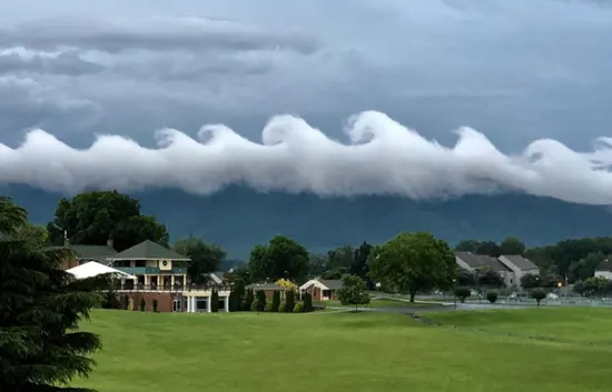
(The Kelvin-Helmholtz cloud.)

Richtmyer-Meshkov Instability: It is considered as the impulsive acceleration limit of Rayleigh-Taylor Instability since it occurs when fluids of two different densities are impulsively accelerated.

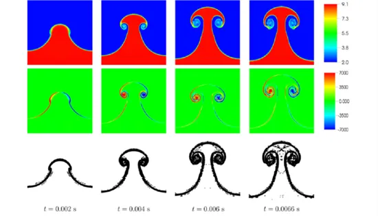
(Time evolution of inviscid Richtmyer-Meshkov Instability.)

Plateau-Rayleigh Instability: Often simply called the Rayleigh instability, it explains why a falling stream of fluid breaks off into smaller portions with the same volume but less surface area. It is an important part of fluid mechanics concerned with ‘fluid thread breakup’.

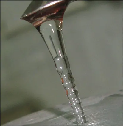
(Development of Plateau-Rayleigh Instability.)

Atwood’s Number (A): It is a dimensionless number in fluid dynamics that is used in the analysis of hydrodynamic instabilities in density stratified flows. It is the ratio of the difference in their mass densities to their sum.
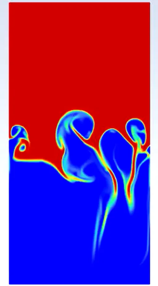
For A close to zero, the instability flows take the form of symmetric fingers of fluids.

For A close to one, the lighter fluid below the heavier fluid takes the form of large,bubble-like plumes.

Atwood number for the case with air as the lighter phase and water as the heavier phase is 0.9975485904.

Atwood number for the case with air as the lighter phase and the user-defined material as the heavier phase is 0.4278357889.

Why a transient-state solver was chosen over the steady-state solver?

Steady-state solvers are used when we are only interested in the end-result. For example, when we have to set up a simulation to calculate the drag force or the lift on an aerodynamic device.

However, when we have to study the time dependence along with the end result, we have to use transient-state solvers. Problems involving combustion, atomisation and interface instabilities such as the Rayleigh-Taylor Instability require the use of a transient-state simulation set-up.

For this problem, as we are studying how the interface collapses due to the instability as a function of time, we have chosen the transient-state solver.

Simulation Set-Up:

This simulation set-up would be a 2D simulation to see how the interface of two liquids, with the denser liquid at the bottom, would behave in the presence of gravity.

This set-up is an important foray into studying multi-phase flows using the 'Volume of Fluid' method.

Geometry set-up:

The sketch plane was opened in SpaceClaim such that the normal to the plane is in the z-direction.

A 20mmX20mm square was drawn and then it was made into a surface using the 'Pull' tool.

This surface was named “lighter” as it would represent the zone with the fluid of lesser density.

Similarly, another surface of similar dimensions was created on top of the existing one. This was named as “denser” as this would represent the zone with the fluid of greater density.

These surfaces were moved to a new component named “final_geometry”.

In the ‘Analysis’ section, the ‘Share Topology’ was set to ‘Share’.

Then from the ‘Workbench’ tab, in the ‘Sharing’ section, the ‘Share’ option was used to create the interface between the two surfaces.

Before meshing, named selections were made. The lighter and denser surfaces were named as they were.

A base line mesh with element size set as 0.5mm was generated.

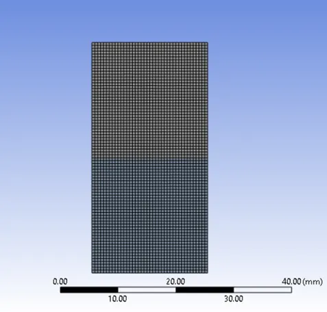
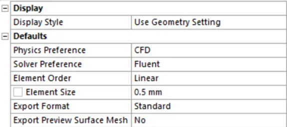
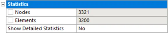
(Mesh details and statistics.)

Solver set-up for base-line run:

The Transient state solver was used for this simulation.

The gravity option was enabled and was set to ‘-9.81m/s’ in the ‘y’-direction.

The energy equation was left unchecked. The viscous turbulence model was set to 'Laminar'.

In the ‘Models’ section, the ‘Multiphase Model’ was chosen.

The ‘Volume of Fluid’ method was selected.

In the ‘Volume Fraction Parameters’, the formulation was set to ‘Implicit’ and the ‘Number of Eulerian Phases’ was set to 2.

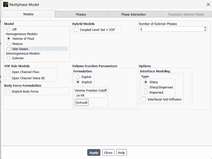
In the ‘Materials’ section, the properties for water (liquid) were copied over from the fluent database.

Back in the ‘Multiphase Model’, in the 'Phases' tab, the primary phase was set to be air and was named as ‘lighter-phase’.

Similarly, the secondary phase was set to be water and was named as ‘denser-phase’.

Now, the solution was initialised in the standard mode. Now, to finish initialising the solution, the zones had to be patched.

In the dialogue box for patching, the ‘Phase’ was set to ‘denser-phase’.

The variable was set to ‘Volume Fraction’.

In the ‘denser’ zone, the value was set to ‘1’ and in the ‘lighter’ zone, the value was set to ‘0’.

Now, the contour to display the volume fraction of the ‘denser-phase’ was created. An animation was also created to capture the changes in the contour with the passage of time.

Now, the size of the time step was set to 0.005 seconds (to maintain a reasonable courant number in accordance with the mesh size). The number of time-steps were set to 1500 and then the solution was calculated.

For the refined mesh, the element size was set to 0.1mm and the time step was proportionally reduced to 0.001 seconds (to maintain the value of the Courant number) and the calculations were carried out again.

[The Courant number is proportional to the time-step and inversely proportional to the mesh element size.]

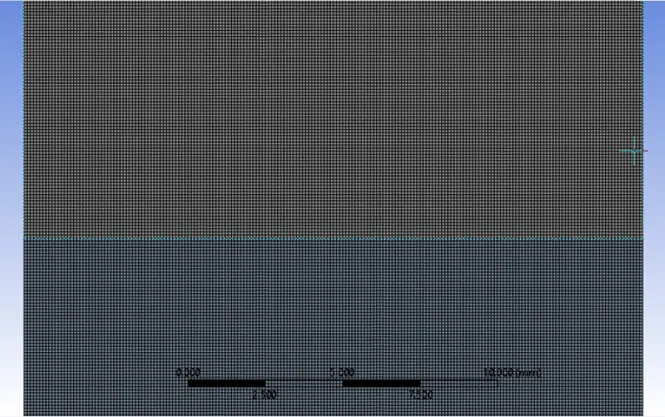
(The mesh is much finer.)

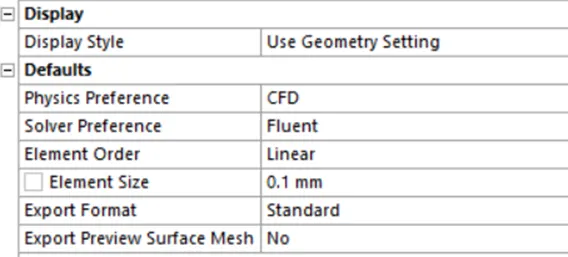
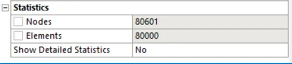
(Mesh details and statistics.)

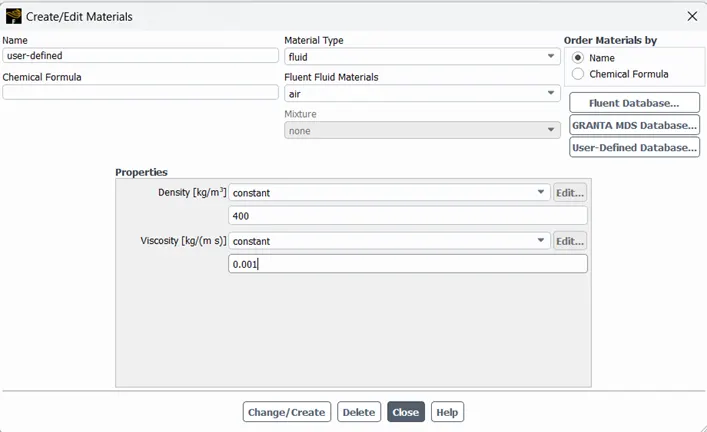
For the second case, a new material with the name ‘user-defined’ was created in the ‘Materials’ section with the given parameters and was set to be the ‘lighter-phase’.

Observations and Conclusions:

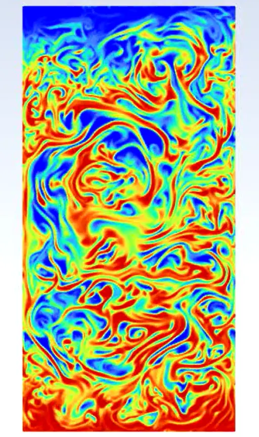
As expected, the coarser mesh provided a very diffused contour. After the collapse of the interface, the contour took on a banded design.

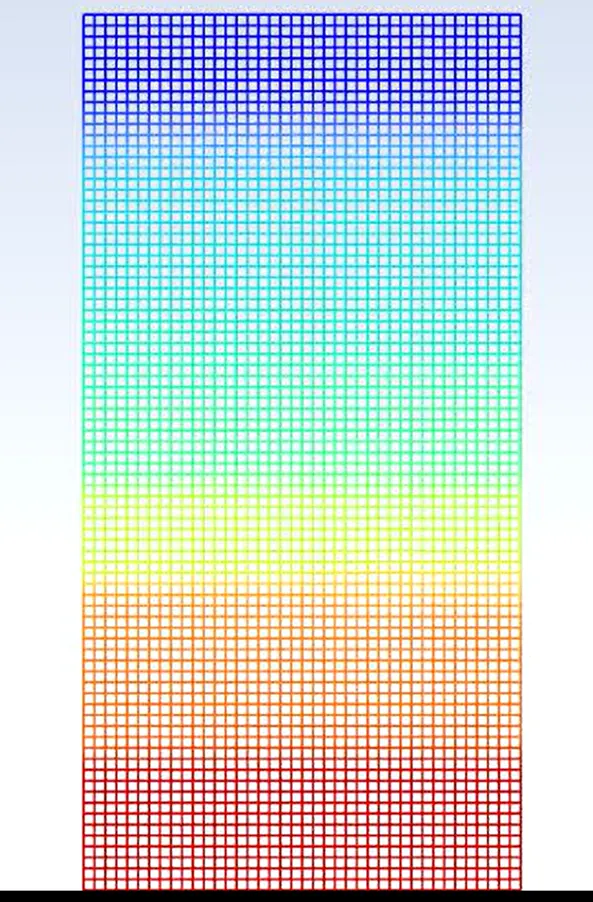
The mesh refinement produced much sharper features on the contours. At the end, the contour did not take on a diffused banded form as for the previous case. It produced a very resolved, sharp and intricate feature.

The Atwood number for this combination of phases was 0.9975485904. Since it was a value close to 1, we see that the lighter fluid below the heavier fluid takes the form of large,bubble-like plumes.

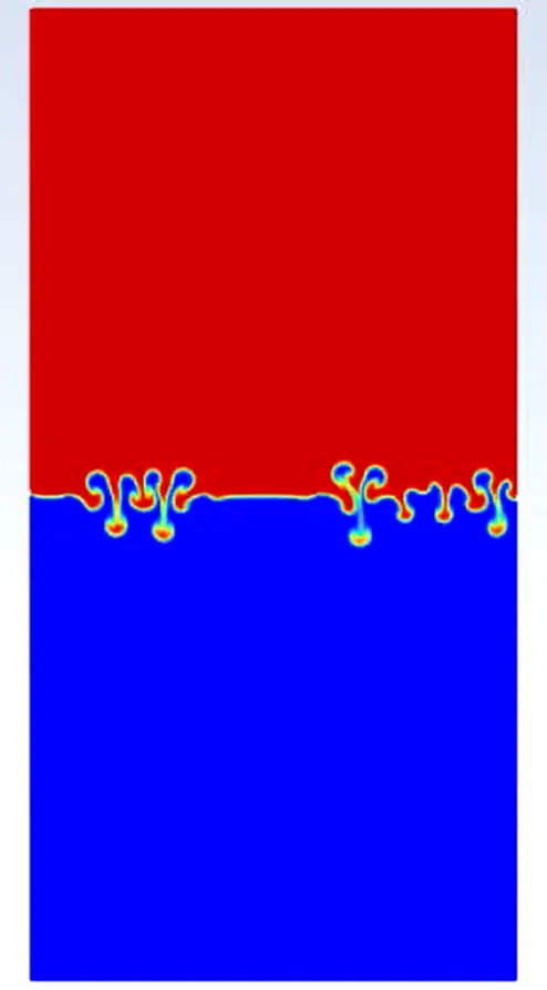
For the user defined material, the Atwood number turned out to be much lower. The Atwood number calculated was 0.4278357889.

As expected, for low Atwood numbers, we observe that the instability flows take the form of symmetric fingers of fluids.

The link to the solution animations: https://drive.google.com/drive/folders/1YKCO7FEuA8Dcj9UgTA5U_EBcRDuJ-QsV?usp=drive_link