Week 5 - Rayleigh Taylor Instability

AIM: Study and Simulation of Rayleigh Taylor Instability using VOF method.

OBJECTIVE:

1. Find some practical CFD models that have been based on the mathematical analysis of Rayleigh Taylor waves.
2. <!-- [if !supportLists]-->To Perform the Rayleigh Taylor instability simulation for 2 different mesh sizes with the base mesh being 0.5 mm.
3. <!-- [if !supportLists]-->To explain why a steady-state approach might not be suitable for these types of simulation. [Choose Air and Water for this simulation.
4. To Run one more simulation with water and user-defined material (density = 400 kg/m³, viscosity = 0.001 kg/m-s) for refined mesh.
5. To define the Atwood Number and to find out the Atwood number for both the cases and explain how the variation in Atwood number in the above two cases affects the behaviour of the instability. 

RAYLEIGH–TAYLOR INSTABILITY INTRODUCTION:

• <!-- [if !supportLists]-->The Rayleigh–Taylor instability, or RT instability (after Lord Rayleigh and G. I. Taylor), is an instability of an interface between two fluids of different densities which occurs when the lighter fluid is pushing the heavier fluid.
• <!-- [if !supportLists]-->Examples include the behavior of water suspended above oil in the gravity of Earth, mushroom clouds like those from volcanic eruptions and atmospheric nuclear explosions, supernova explosions in which expanding core gas is accelerated into denser shell gas, instabilities in plasma fusion reactors and inertial confinement fusion.

Explanation:

• Water suspended atop oil is an everyday example of Rayleigh–Taylor instability, and it may be modeled by two completely plane-parallel layers of immiscible fluid, the denser fluid on top of the less dense one and both subject to the Earth's gravity. The equilibrium here is unstable to any perturbations or disturbances of the interface: if a parcel of heavier fluid is displaced downward with an equal volume of lighter fluid displaced upwards, the potential energy of the configuration is lower than the initial state. Thus, the disturbance will grow and lead to a further release of potential energy, as the denser material moves down under the (effective) gravitational field, and the less dense material is further displaced upwards. This was the set-up as studied by Lord Rayleigh. The important insight by G. I. Taylor was his realization that this situation is equivalent to the situation when the fluids are accelerated, with the less dense fluid accelerating into the denser fluid. 

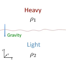
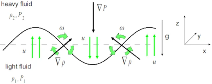
Practical CFD models that have been based on mathematical analysis of RT waves...

1. <!-- [if !supportLists]-->Kelvin-Helmholtz instability
2. <!-- [if !supportLists]-->Richtmyer-Meshkov instability
3. <!-- [if !supportLists]-->Plateau-Rayleigh instability

Kelvin-Helmholtz instability:

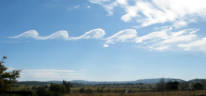
• This instability typically occurs when there is velocity shear in a single continuous fluid, or additionally where there is a velocity difference across the interface between two fluids. Kelvin-Helmholtz instabilities are visible in the atmospheres of planets and moons, such as in cloud formations on Earth or the Red Spot on Jupiter, and the atmospheres of the Sun and other stars.

Richtmyer–Meshkov instability

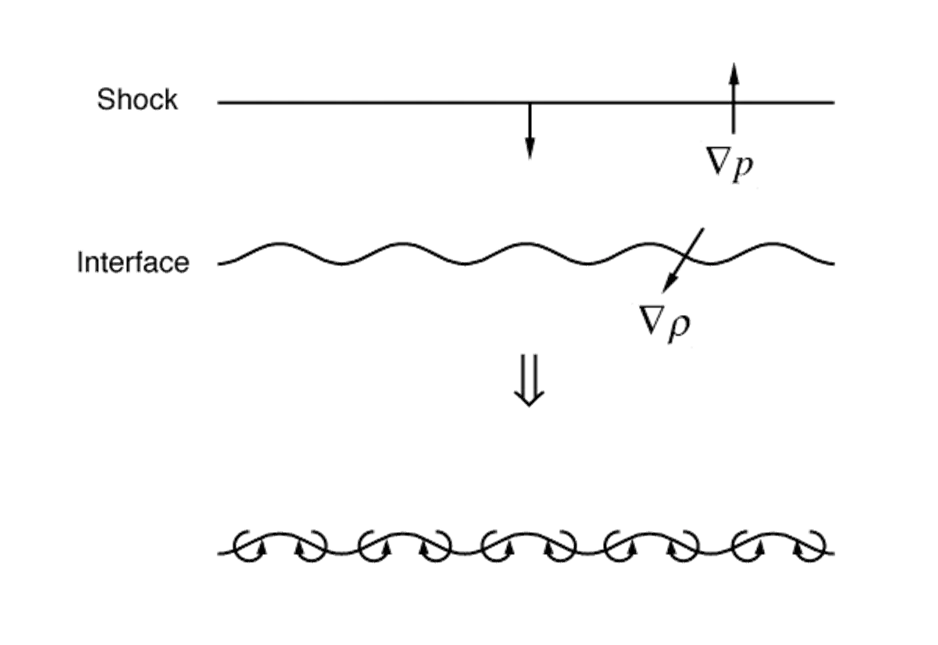
• Richtmyer–Meshkov instability is the fluid flow phenomenon that occurs when a shock wave impinges (in the normal direction) upon an interface separating two gases having different densities. The instability causes perturbations on the interface to grow, producing vortical structures which potentially result in a turbulent mixing layer, as illustrated in Figure

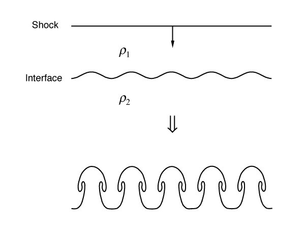
• Although the shock interaction process is inherently compressible, Richtmyer–Meshkov instability can also be produced by the impulsive acceleration of two incompressible fluids. In this sense, Richtmyer–Meshkov instability is related to the better known Rayleigh–Taylor instability, and is often referred to as impulsive Rayleigh–Taylor instability. The physical mechanism producing the instability is most easily described using the dynamics of the vorticity field ω=∇×v . Vorticity is deposited on the perturbed interface by the misalignment of the pressure gradient of the shock wave and the density gradient at the fluid interface.

 Plateau–Rayleigh instability:

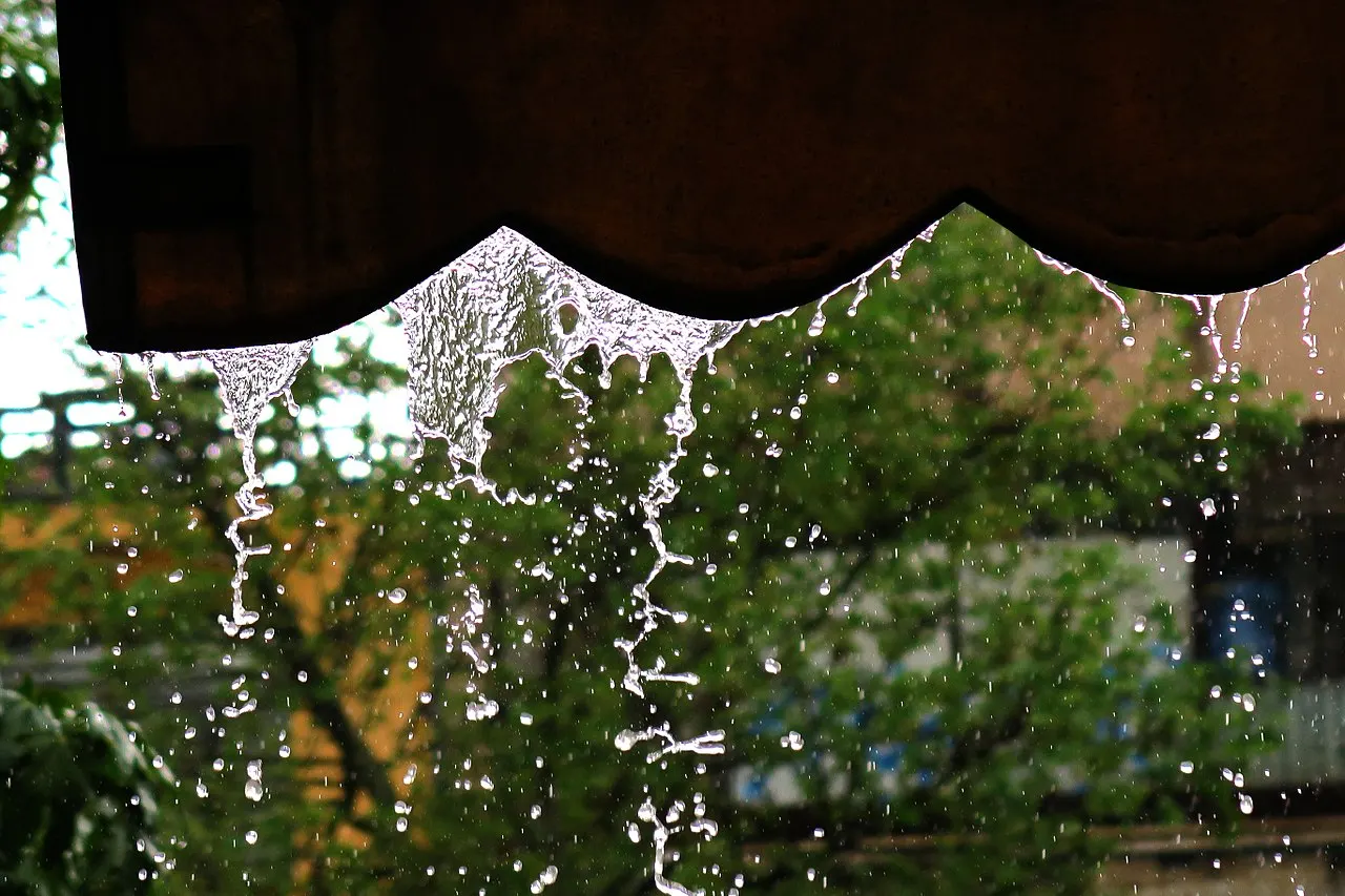
• The Plateau–Rayleigh instability, often just called the Rayleigh instability, explains why and how a falling stream of fluid breaks up into smaller packets with the same volume but less surface area. It is related to the Rayleigh–Taylor instability and is part of a greater branch of fluid dynamics concerned with fluid thread breakup. This fluid instability is exploited in the design of a particular type of ink jet technology whereby a jet of liquid is perturbed into a steady stream of droplets. The driving force of the Plateau–Rayleigh instability is that liquids, by virtue of their surface tensions, tend to minimize their surface area.
• A special case of this is the formation of small droplets when water is dripping from a faucet/tap. When a segment of water begins to separate from the faucet, a neck is formed and then stretched. If the diameter of the faucet is big enough, the neck does not get sucked back in, and it undergoes a Plateau–Rayleigh instability and collapses into a small droplet.

ATWOOD NUMBER:

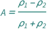
The Atwood number is a dimensionless number in fluid dynamics used in the study of hydrodynamic instabilities in density-stratified flows.The Atwood number equals the ratio of the difference in mass densities to their sum.

Formula

• For the case of small Atwood number, the density difference between the two sides of the interface is small, and the density distribution of the upper and lower layers is nearly symmetrical. The initial density stratification plays a dominant role, and the expansion-compression effect has little influence.
• With the increase in the Atwood number, the stabilization effect of initial density stratification decreases, and the instability caused by the expansion-compression effect becomes more significant. The flow structures of bubbles and spikes are quite different at medium Atwood number. The effect of compressibility on the bubble velocity is strong at large At. The bubble height is approximately a quadratic function of time at potential flow growth stage. The average bubble acceleration is nearly proportional to the square of Mach number at At = 0.9.

Atwood number for water and air is 0.997

Atwood number for water and userdefined material is 0.427

RAYLEIGH TAYLOR INSTABILITY SIMULATION FOR DIFFERENT MESH SIZE

Geomentry creation in spaceclaim

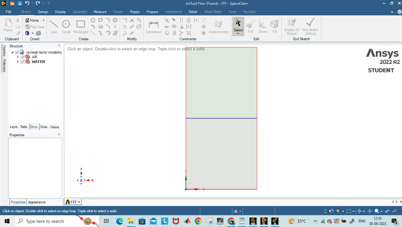
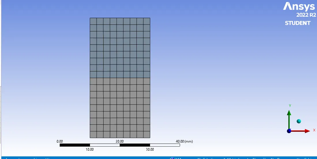
Two 2D domains (square of side 20 mm) with a common edge are created in Spaceclaim to hold the two phases. The two domains are shared using the 'share' option under the workbench tab in SpaceClaim in order to create a conformal mesh.

Baseline mesh creation:

Fluent setup process:

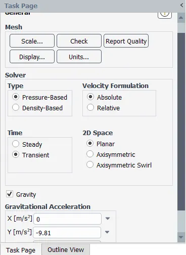
• A pressure-based, transient solver is used. The transient solver is chosen to capture the instability at the interface that collapses with respect to time. Gravity is enabled. The acceleration due to gravity is set to -9.81m/s^2 in the Y-direction. Negative sign indicates that movement of fluid is in the opposite direction to gravity.
• A steady-state VOF simulation makes sense only when there are distinct inlet boundaries for different phases.
• Under viscous models, the Laminar option is chosen, as the flow is essentially laminar.
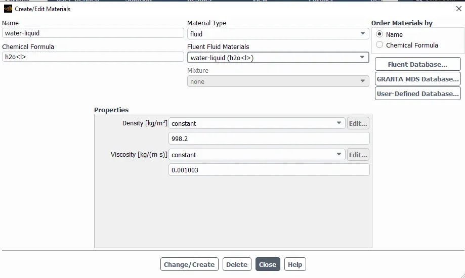
• From the material library, air and water are chosen. The material properties are constant and do not change. 

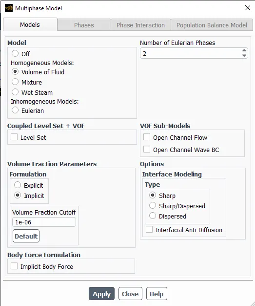
The multiphase model is clicked, and the volume of fluid method is chosen. The number of eulerian phases is set to 2. The Implicit is chosen as the problem is a transient one. The material of the primary phase (air) and the secondary phase is selected (water). The material can be chosen in the other way round also.

CASE 1: SIMULATION FOR THE MESH SIZE OF 0.5MM

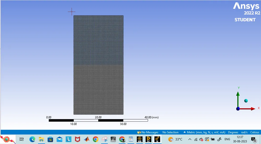
Since the geometry is very simple and consists of straight lines, the default mesh generated is of square type. The base mesh size used for the problem is 0.5 mm. The total cell count, in this case, is 3200.

Contour for 0.5mm mesh size:

Animation video link for 0.5mm baseline mesh:

animation-normal-meshing.mpeg

https://1drv.ms/v/s!AmEqYh6drZjVoD0VRQMmRk6dZYxT?e=Wi3bZs

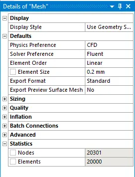
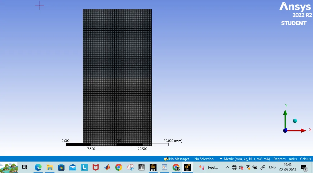
CASE 2: SIMULATION FOR THE MESH SIZE OF 0.2MM

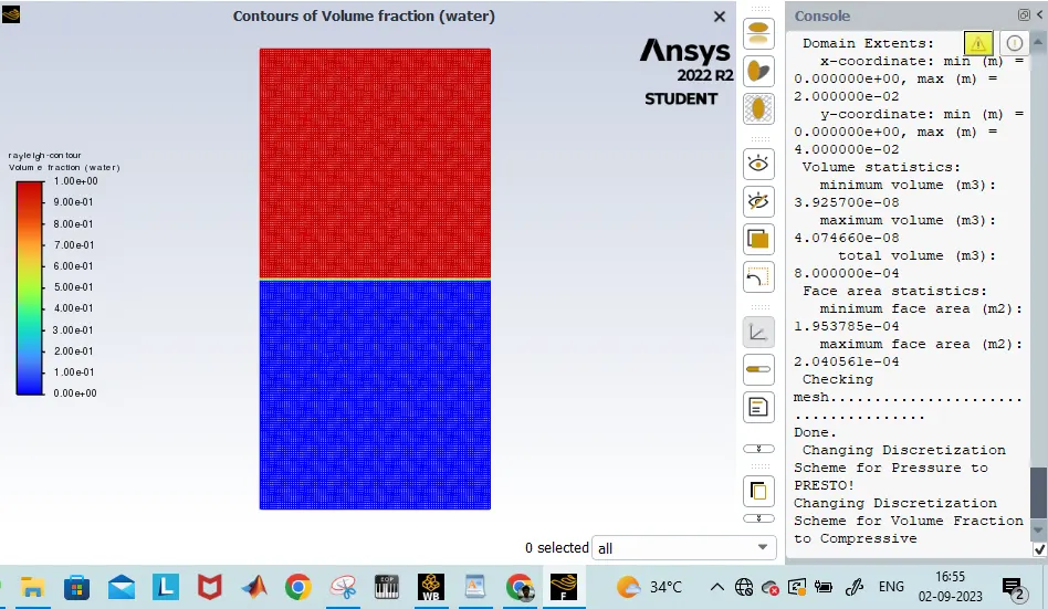
Contour for 0.2mm mesh size:

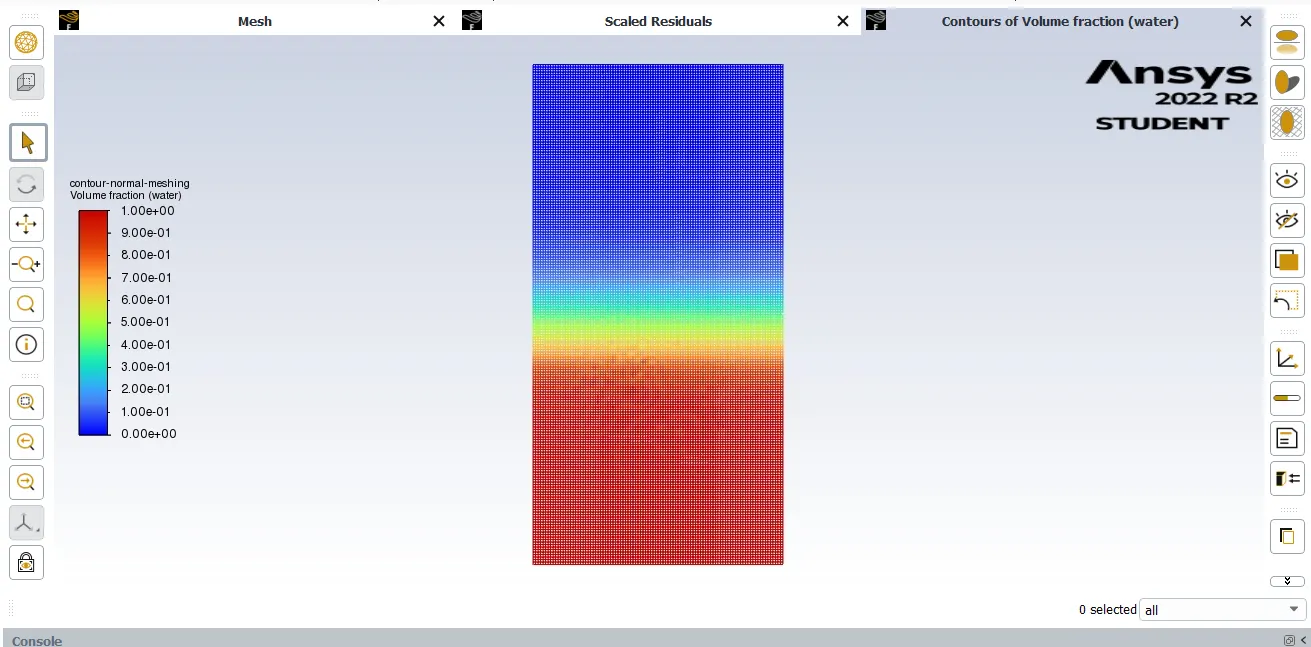
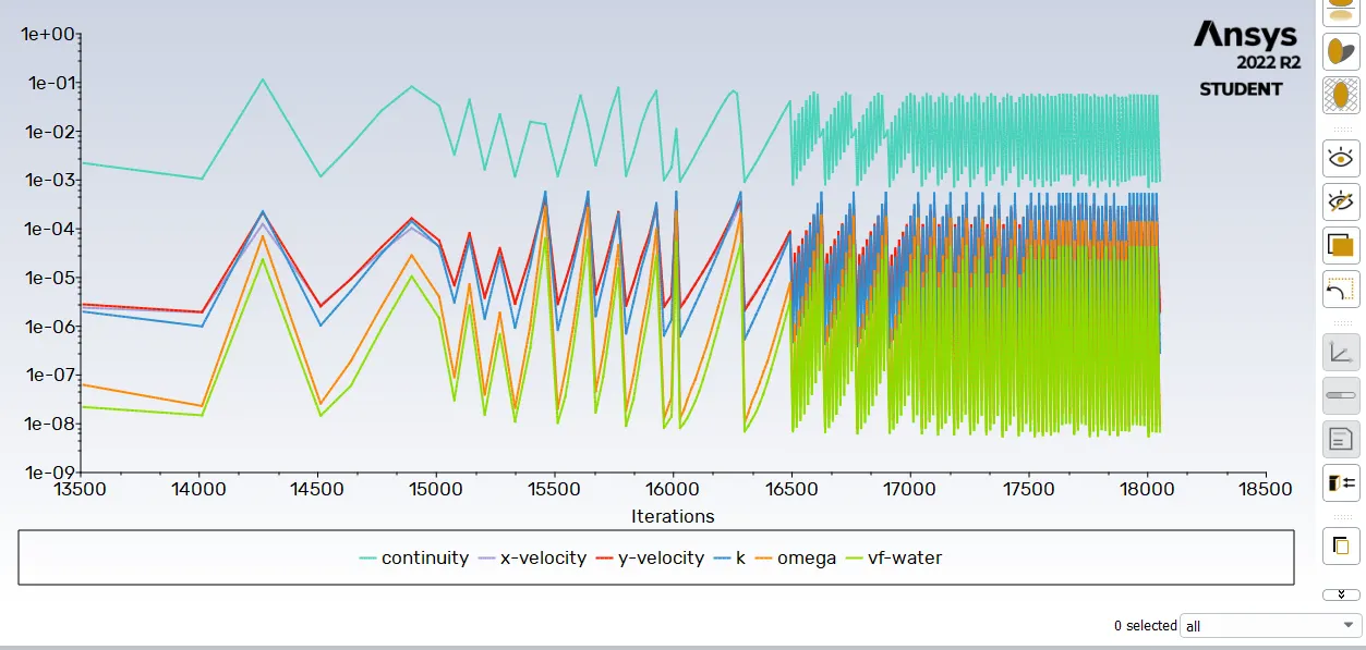
Residual plot:

Animation video link for mesh refinement of 0.2mm:

animation-meshrefinement.mpeg

https://1drv.ms/v/s!AmEqYh6drZjVoD5EaLcUkqblvQtS?e=p96HnY

CASE 3: SIMULATION WITH USER DEFINED MATERIAL (MESH SIZE OF 0.2MM)

User defined material ( Change density and viscosity for air)

1. Density = 400 kg/m³
2. viscosity = 0.001 kg/m-s

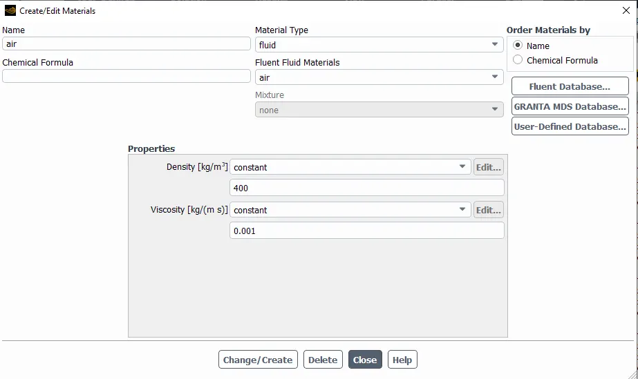
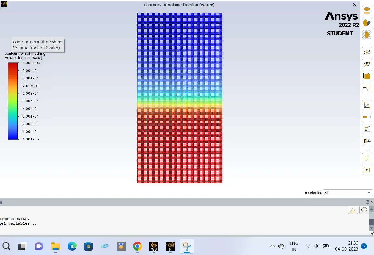
Contour for user-defined material

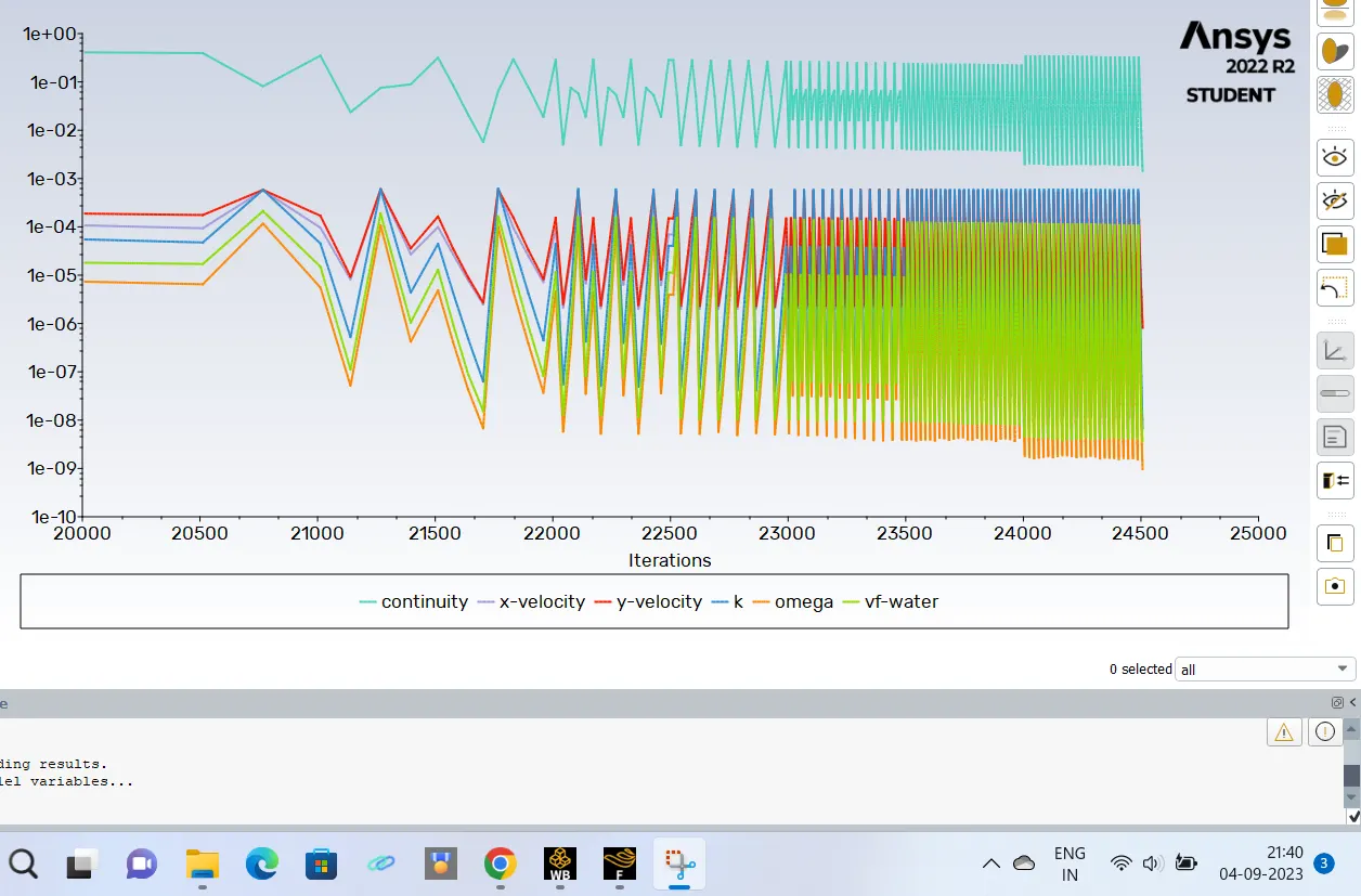
Residuals for user-defined material and water

Animation video link for userdefined material with mesh element size of 0.2mm:

https://1drv.ms/v/s!AmEqYh6drZjVoD_7ca-MZVGrLTQE?e=asFus2

animation-userdefined material.mpeg

RESULT:

Case 1:

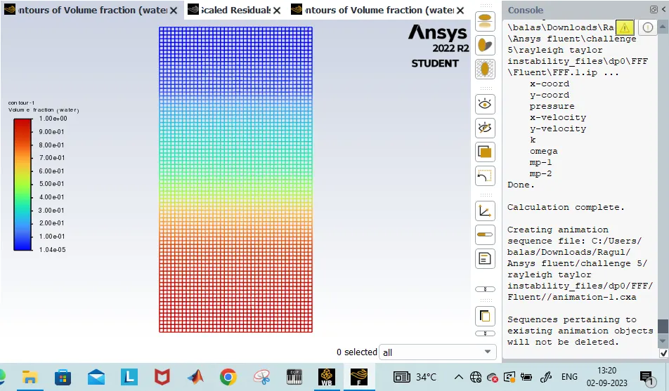
• The instability of the interface is observed in the animation. The heavier fluid settles at the bottom, and the lighter fluid settles on top. The middle of the domain is taken over by cells containing an equal amount of both phases. Bands of other volume fractions can also be observed from the contour.
• The instabilities start off as straight line and immediately takes the shape of mushroom clouds with the lighter fluid (air) penetrating the heavier fluid. This penetration of the lighter fluid into the heavier fluid grows deeper and a series of shapes are patterns are formed. Swirl-like patterns are formed in the flow. They are observed to be single layered.

Case 2:

• The development of the instability becomes more clearer with refinement in the mesh. The patterns formed are mostly swirling. They diffuse and transport the lighter fluid into the heavy fluid.
• The magnitude of perturbation is observed to be more intense. The sizes of the swirl are much larger. This refined case takes much more time to settle compared to the baseline. Even after settling, small bubble-like formations are observed.

Case 3:

• The density difference between the two fluids is reduced. It is observed that the intensity of instability of the interface is relatively reduced. The swirls are smaller in size, are more in number, and are observed for a longer duration. The bubble-like formation becomes more prominent and is constantly in motion even at the end of the simulation. 

CONCLUSTION:

• The Rayleigh Taylor Instability is carried out using the Volume of Fluid (VOF) technique and a transient solver. The Atwood number is defined.
• The instability is very sensitive wrt the time step and the mesh size. Convergence of simulation took lot of time 
• With refinement in the mesh, the instability patterns are more clear.
• With the increase in Atwood number, the intensity of the instability increases, and the time taken for the instability to settle down decreases.