Week 5 - Rayleigh Taylor Instability

1. Rayleigh Taylor (RT) Instability

Rayleigh Taylor instability is a fluid instability phenomenon that occurs at the interface between two fluids of different densities, with the lighter fluid pushing into the denser fluid under the influence of gravity. The mathematical analysis of Rayleigh-Taylor waves has provided insights into the behavior of this instability, and these mathematical models have been adapted for CFD calculations in various practical applications.

Practical CFD Models

Several practical CFD models have been developed based on the mathematical analysis of Rayleigh Taylor waves. Here arw few examples:

1. Level Set Methods: Level set methods are commonly used in CFD simulations to model and analyze RT instabilities. These methods represent the interface between two fluids using a scalar function that evolves over time. By solving the level set equation, the growth and behavior of RT waves can be simulated and studied.

2. Volume-of-Fluid (VOF) Methods: VOF methods are another approach for modeling RT instabilities. These methods track the interface between two fluids by dividing the computational domain into discrete control volumes. By solving the conservation equations for each fluid phase, the growth and evolution of RT waves can be simulated.

3. Smoothed Particle Hydrodynamics (SPH): SPH is a meshless Lagrangian method that has been used to study RT phenomena. It approximates fluid properties using particles and computes fluid dynamics based on the interactions between particles. SPH has been employed to model complex RT flows, including multiphase and compressible scenarios.

4. Large Eddy Simulation (LES): LES is a technique that resolves large scale turbulent structures while modeling the effects of smaller scale turbulence. LES has been applied to study RT mixing and turbulence characteristics, providing insights into the behavior of RT waves in turbulent flows.

Mathematical models used in CFD are adapted to facilitate numerical calculations by discretizing the governing equations and implementing numerical methods. Here is an explanation of how these mathematical models are adapted for CFD calculations:

1. Discretization: The continuous governing equations, such as the Navier-Stokes equations, are discretized into a set of algebraic equations that can be solved numerically. This involves dividing the computational domain into a mesh or grid composed of discrete control volumes or elements.

2. Numerical Methods: Various numerical methods are employed to solve the discretized equations. Commonly used methods include finite difference, finite volume, finite element, and spectral methods. These methods approximate derivatives and integrals, allowing the equations to be solved iteratively on the discrete grid.

3. Boundary Conditions: Boundary conditions are specified to represent the physical constraints at the boundaries of the computational domain. These conditions may include specifying the inflow/outflow velocities, pressure, temperature, or other relevant properties. The choice of boundary conditions depends on the specific problem being solved.

4. Time Marching: For transient simulations, a time-marching scheme is employed to advance the solution in time. Various schemes, such as explicit or implicit methods, can be used to update the solution at each time step.

5. Turbulence Modeling: Turbulence models are incorporated to simulate turbulent flows. These models provide closure for the unresolved turbulence scales, allowing the simulation to capture the effects of turbulence on the flow behavior. Different turbulence models, such as Reynolds-averaged Navier-Stokes (RANS) or Large Eddy Simulation (LES), can be applied depending on the required level of accuracy and computational resources.

By adapting mathematical models for CFD calculations, engineers and scientists can simulate and analyze a wide range of fluid flow phenomena to gain insights, make predictions, and optimize designs.

2. Simulation Process

The model for the simulation is prepared in ANSYS SpaceClaim.

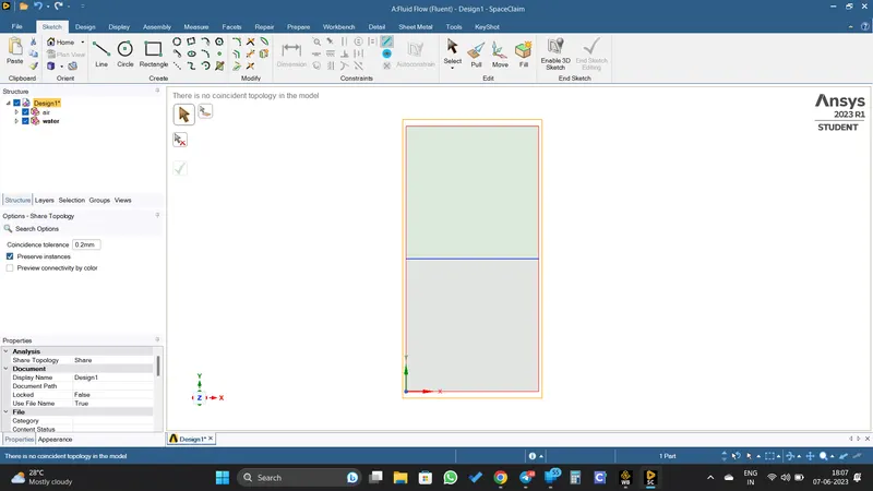
Then the model is meshed.

Mesh size 0.5 mm

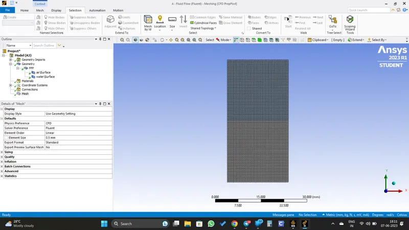
No: of nodes: 3321

No: of elements: 3200

Then the meshed model is opened in ANSYS Fluent

Setup Parameters;

Viscous Model: Laminar

Solver Type: Pressure Based

Solver Time: Transient

Gravity: Enabled in -Y direction (9.81 `m`/`s^2`)

Multiphase;

• Model: Volume of fluid (VOF)
• Volume Fraction Formulation: Implicit
• No: of Eulerian Phases: 2

Materials;

• Fluid Type: Air (Primary Phase) & Water (Secondary Phase)
• Solid Type: Aluminum

Solution Initialization Patch;

• Phase - Water (Value of volume fraction = 1)
• Phase - Air (Value of voulme fraction = 0)

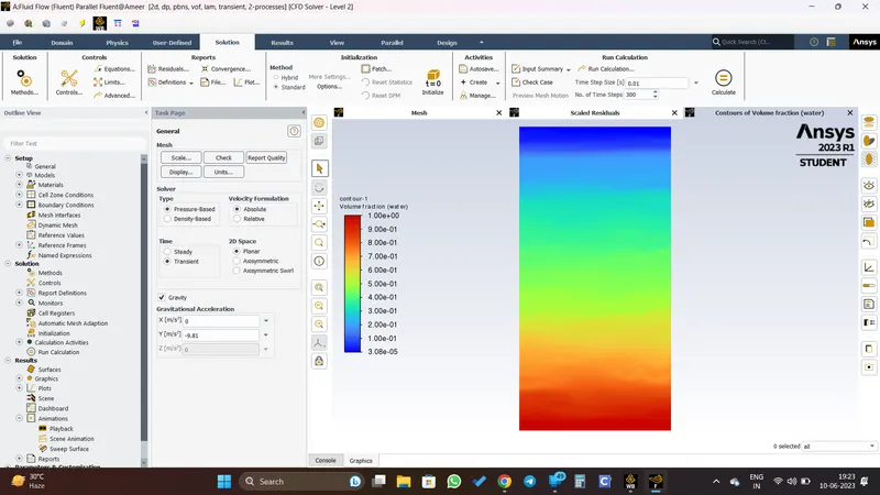
Created contour of phases and the solution animation.

Then the setup is ran

RESULTS

Scaled Residuals

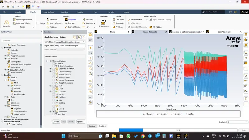
Contour Of Volume Fraction (water)

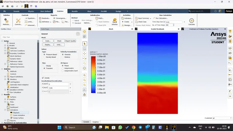
Solution Animation

For Solution animation, click here

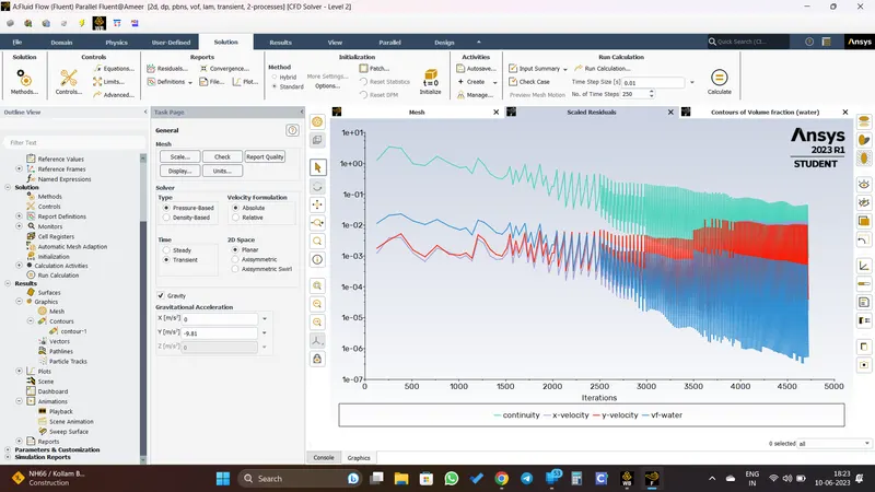
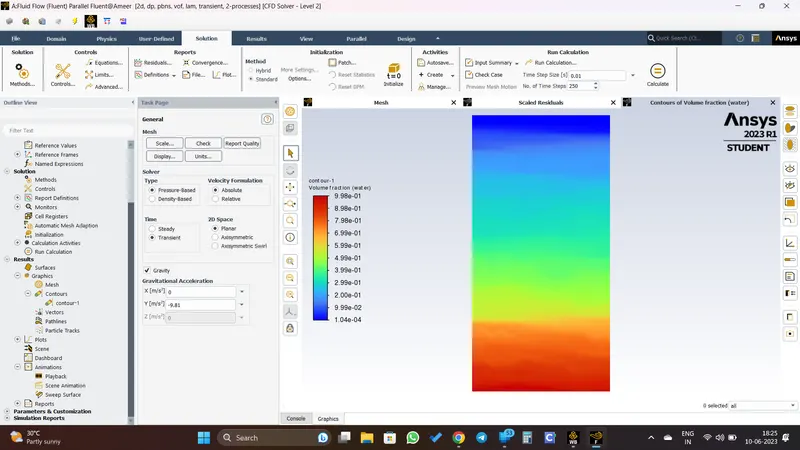
The model is refined by meshing with 0.3 mm element size.

Setup parameters are kept same.

RESULTS

Scaled Residuals

Contour Of Volume Fraction (water)

Solution Animation

For Solution animation, click here

Effect Of Mesh Size On Simulation

The mesh size plays a crucial role in accurately capturing the behavior of Rayleigh Taylor instabilities.

RT instabilities involve the formation and evolution of complex flow structures, including spikes, bubbles, and mixing layers. To accurately capture these features, the mesh size should be fine enough. Smaller mesh elements allow for better representation of the interfacial dynamics and the small scale structures that develop during the growth of the instability.

The finer mesh helps maintain the sharpness of the interfacial region between the two fluids.

Why A Steady State Approach Might Not Be Suitable?

A steady state approach, where the flow variables do not change with time, might not be suitable for simulating Rayleigh Taylor instabilities for the following reasons:

1. Transient Nature: RT instabilities are inherently transient phenomena that evolve over time. The mixing and interaction between fluids with different densities result in complex flow patterns that continually change as the instability progresses. A steady-state approach would not capture the dynamic evolution and time-dependent behavior of the instability accurately.

2. Unsteady Flow Features: RT instabilities involve the interplay of buoyancy, vorticity, and turbulence, leading to the development of intricate flow features such as roll-up vortices, spikes, and bubbles. These flow features are highly unsteady in nature and require a transient simulation to capture their formation, evolution, and interaction accurately.

3. Instability Growth: The growth of RT instabilities is a crucial aspect to understand and predict. The amplification of the instability occurs over time as the less dense fluid rises and the denser fluid falls, leading to the interfacial deformation. A steady-state approach would not account for the time-dependent growth and development of the instability, limiting the ability to study its characteristics accurately.

4. Turbulent Mixing: Turbulence plays a significant role in the mixing process associated with RT instabilities. Turbulent eddies and vortices enhance the interfacial mixing between the fluids, resulting in a complex mixing zone. Capturing the turbulent characteristics and its impact on mixing necessitates a transient simulation to accurately represent the time-varying turbulent flow field.

5. Transition to Turbulence: The transition from laminar to turbulent flow is often observed in RT instabilities as the flow becomes more chaotic and intricate. This transition process is intrinsically time-dependent, and a steady-state approach would not adequately capture the dynamic nature of the transition and its associated effects on the instability.

3. Simulation With Water And User-Defined Material

The material properties are set as per the given question.

Mesh element size 0.03 mm

All the other setup parameters are kept same.

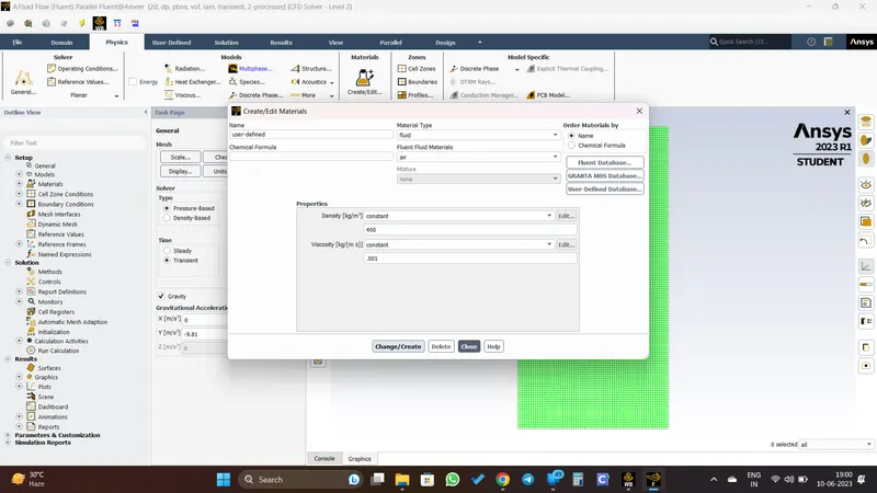
RESULTS

Scaled Residuals

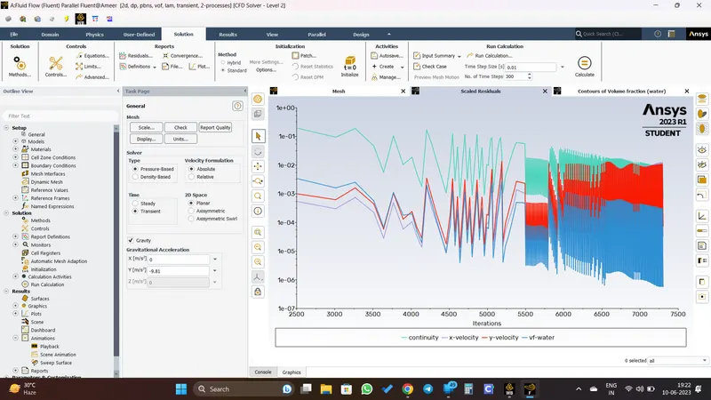
Contour Of Volume Fraction (water)

Solution Animation

For Solution animation, click here

Atwood Number

The Atwood number is a dimensionless parameter used to quantify the density difference between two fluids in a flow system. It is named after the British physicist George Atwood, who first introduced the concept. The Atwood number is denoted by the symbol "A" and is defined as the ratio of the density difference between the fluids to the average density:

Atwood number (A) = (ρ2 - ρ1) / (ρ2 + ρ1)

where: ρ1 = density of the first fluid

ρ2 = density of the second fluid

The Atwood number ranges from -1 to 1, representing different density configurations:

• When A = -1, the fluids are completely reversed in density, with the denser fluid above the lighter fluid.
• When A = 0, the densities of the two fluids are equal.
• When A = 1, the denser fluid is below the lighter fluid.

The Atwood number provides a measure of the buoyancy forces and the resulting instability that can arise when there is a density difference in a flow system. It is particularly relevant in studying phenomena such as Rayleigh-Taylor instabilities and Richtmyer-Meshkov instabilities, where the interface between the fluids becomes unstable and leads to mixing and complex flow patterns.

In summary, the Atwood number quantifies the relative density difference between two fluids in a flow system and is used to characterize and analyze buoyancy driven instabilities.

Here's an explanation of how the Atwood number affects the instability:

1. Growth Rate: The Atwood number directly influences the growth rate of the instability. In general, a higher Atwood number corresponds to a higher growth rate, meaning that the instability develops more rapidly. A lower Atwood number leads to a slower growth rate and a less pronounced instability.

2. Mixing Zone: The Atwood number affects the depth and extent of the mixing zone between the two fluids. A higher Atwood number typically results in a more extensive mixing zone with increased interpenetration and mixing of the fluids. Conversely, a lower Atwood number leads to a narrower mixing zone with less mixing between the fluids.

3. Instability Mode: The Atwood number also influences the dominant instability mode. For small Atwood numbers, the instability is primarily driven by the Rayleigh-Taylor mode, where buoyancy is the main destabilizing force. As the Atwood number increases, additional instability modes such as the Richtmyer-Meshkov and Kelvin-Helmholtz modes may become significant, introducing additional complexities to the flow patterns.

4. Transition to Turbulence: The Atwood number can determine the transition from laminar to turbulent behavior in the flow. Higher Atwood numbers tend to promote the onset of turbulence earlier in the development of the instability. Turbulence can significantly enhance mixing and lead to increased complexity in the flow dynamics.

5. Front Propagation: The Atwood number affects the propagation speed of the RT instability front. A higher Atwood number results in faster front propagation, while a lower Atwood number leads to slower front propagation.

Effects Of Atwood Number In The Above Two Cases

CASE	MESH SIZE	NO: OF ELEMENTS	ATWOOD NUMBER
CASE 1.1	0.5	3200	0.997
CASE 1.2	0.3	8978	0.997
CASE 2 (UDF)	0.3	8978	0.428

From the table we can see that, for the setup with the user defined material have low Atwood Number compared to the Water and Air.

While comparing the solution animation of both the case, we can see that the case 2 (case with low Atwood Number) has increased instability and turbulence. Also it has the enhanced mixing and forms complex flow pattern.

For Project File, Click here