Week 5 - Rayleigh Taylor Instability

Aim: To Conduct A Rayleigh Taylor Instability Using Ansys Fluent.

Objective:

• CFD models that have been based on the mathematical analysis of Rayleigh Taylor waves
• To explain these mathematical models have been adapted for CFD calculations.
• To perform the Rayleigh Taylor instability simulation for 2 different mesh sizes with the base mesh being 0.5 mm.
• Compare the results by showing the animations.
• Explain why a steady-state approach might not be suitable for these types of simulation.
• Run one more simulation with water and user-defined material(density = 400 kg/m³, viscosity = 0.001 kg/m-s) for refined mesh.
• Define the Atwood Number.
• The Atwood number for both the cases and explain how the variation in Atwood number in the above two cases affects the behavior of the instability.
  
  

We are doing analysis on these three cases.

• Case 1: Mesh size is 0.5mm for water and air.
• Case 2: Mesh size is 0.2mm for water and air.
• Case 3: Mesh size is 0.2mm for water and user defined fluid.

Theory:

• The Rayleigh-Taylor instability is a fluid instability phenomenon that occurs at the interface between two fluids of different densities when the denser fluid is supported above the lighter fluid. This instability leads to the mixing and interpenetration of the two fluids.
• The instability is named after Lord Rayleigh and G.I. Taylor, who independently studied and explained its behavior. It is a common phenomenon observed in various natural and engineered systems, including fluid dynamics, astrophysics, and plasma physics.
• The Rayleigh-Taylor instability occurs when there is an initial perturbation or disturbance at the interface between the two fluids. Gravitational forces act differently on the two fluids due to their density difference, leading to the development of complex fluid motions and the formation of characteristic structures such as spikes, bubbles, and mushroom-like shapes.
• The instability can be explained using basic physics principles. When a denser fluid is placed above a lighter fluid, gravity tries to pull the denser fluid downwards, while buoyancy opposes this motion. If a small perturbation is present at the interface, it can grow and amplify due to the competition between these forces, leading to the intermixing of the two fluids.
• The Rayleigh-Taylor instability has significant implications in various fields. For example, it plays a crucial role in understanding the behavior of supernovae explosions, where the explosion ejecta interact with the surrounding medium. In inertial confinement fusion research, it can affect the implosion dynamics of fuel capsules. In addition, the instability has applications in engineering, such as mixing processes and atomization in fluid mechanics.
  
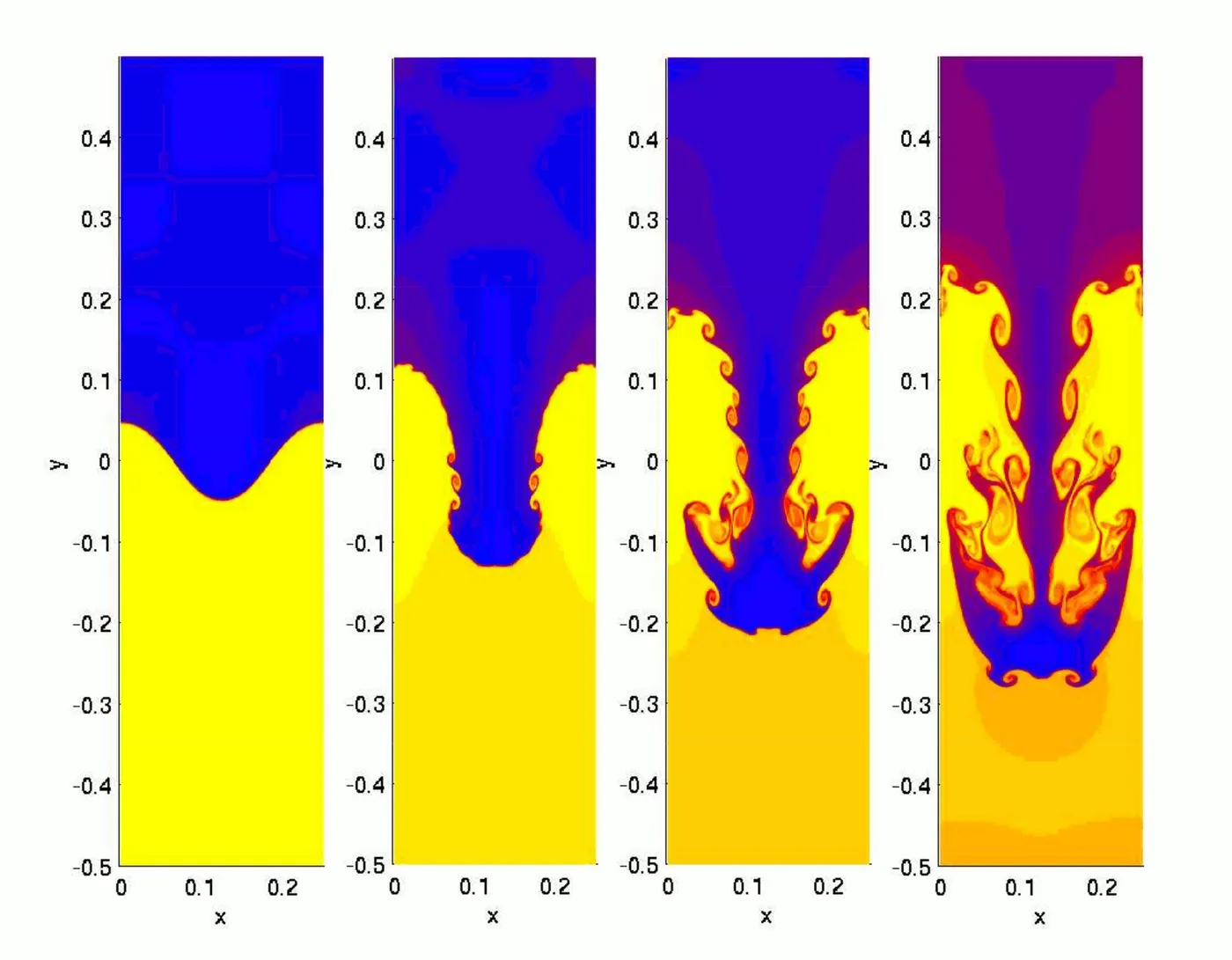
• Animation of fluid mixing
  
  
  

Mathematical models have been adapted for CFD calculations of Rayleigh Taylor.

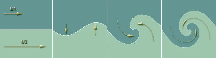
1. Kelvin Helmholtz instability:
   • Is traditionally viewed as an initial-value problem, wherein wave perturbations of a two-layer shear flow grow over time into bil- lows and eventually generate vertical mixing. Yet, the instability can also be viewed as a boundary-value problem.
   • A fluid mechanics is the instability at the interface between two horizontal parallel streams of different velocities and densities, with the heavier fluid at the bottom. This is called Kelvin–Helmholtz instability.
     
     
     
2. Plateau-Rayleigh instability:
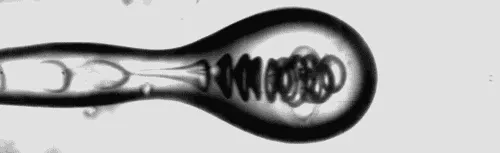
   • The Plateau–Rayleigh instability is named for Joseph Plateau and Lord Rayleigh. In 1873, Plateau found experimentally that a vertically falling stream of water will break up into drops if its length is greater than about 3.13 to 3.18 times its diameter, which he noted is close to `pi`.
   • The Plateau-Rayleigh Instability describes the phenomenon where a falling jet or cylinder of fuid (such as water) at one point ceases to be a jet and breaks into multiple droplets of smaller total surface area.
     
     
     
3. Richtmyer-Meshkov instability
   • Rayleigh-Taylor instability (RTI) is the interpenetration of materials that occurs whenever a light fluid pushes on a heavy fluid. It is a dynamic process whereby the two fluids seek to reduce their combined potential energy.
   • the behavior of water suspended above oil in the gravity of Earth, mushroom clouds like those from volcanic eruptions and atmospheric nuclear explosions, supernova explosions in which expanding core gas is accelerated into denser shell gas, instabilities in plasma fusion reactors and inertia.
   • This instability occurs where there is a velocity shear or velocity difference between the interface of the two fluids. This occurs when two fluids of different density are impulsively accelerated. Normally this is by the passage of a shock wave.
     

Simulation setup:

• Geometry setup:
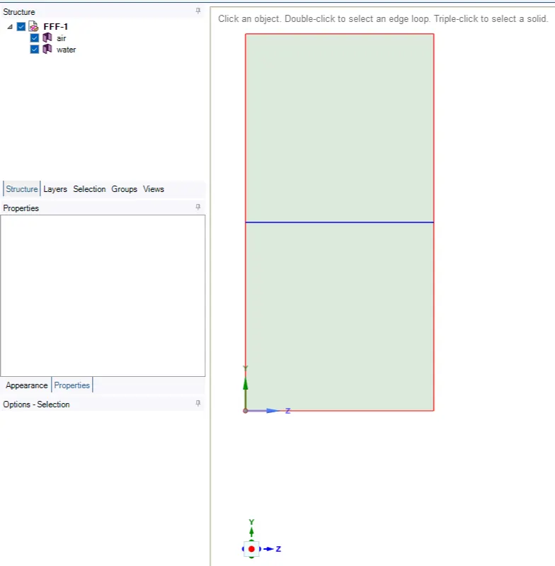
  Created a box for the simulation.
  
  • The upper box is for water, and the lower box is for air.
  • We had used a sharing tool to merge both boxes together.
    
    
• Meshing
  
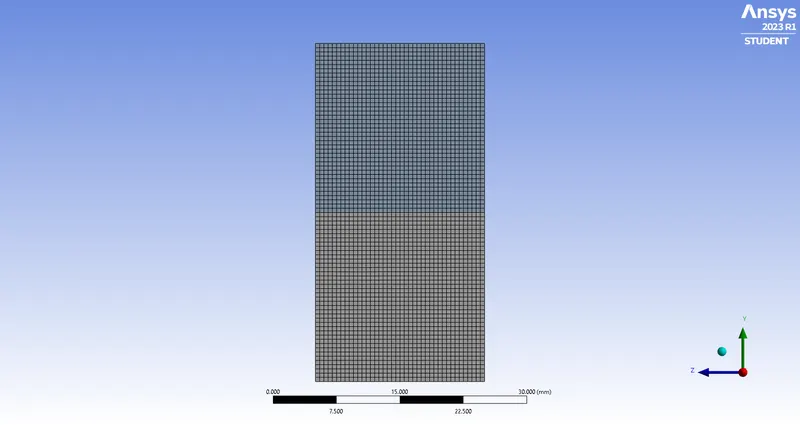
  • Case 1: Base line mesh of 0.5mm.
    • Number of nodes is 3321.
    • The number of elements is3200.
      
      
      
• Setup
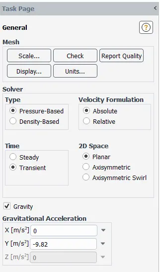
  • General setup
    
    
    
    
    
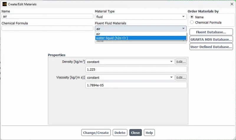
  • Material
    
    
    
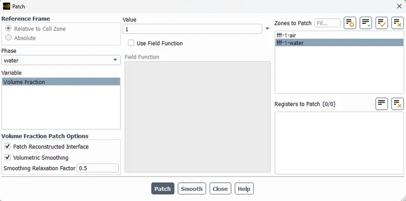
  • Patching a setup for mixture of air and water.
    
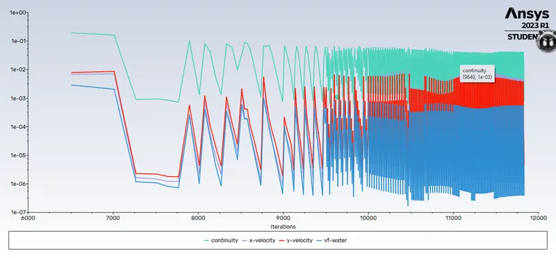
  • Scaled Residuals
    
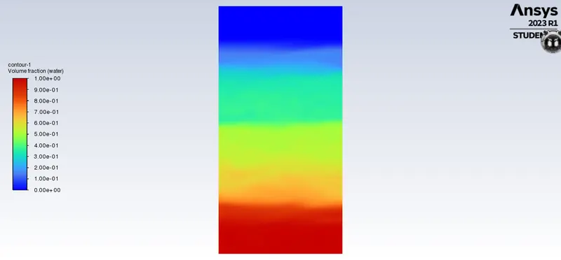
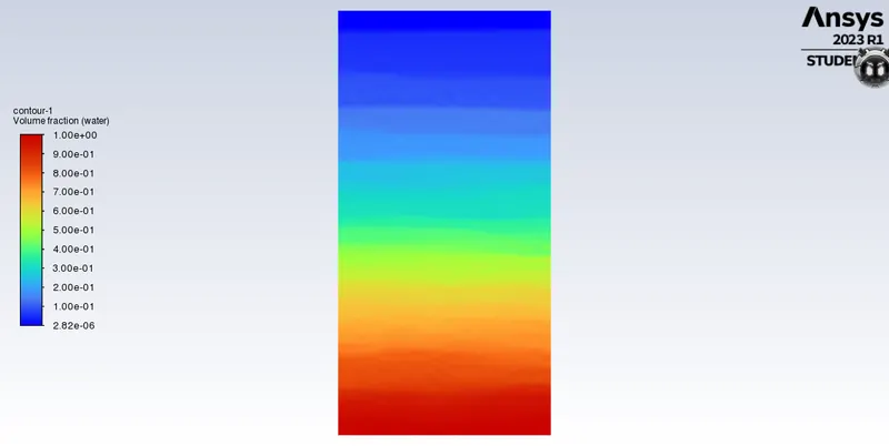
  • Contours of volume fraction
    
    
    
  • video link
    https://youtu.be/GYSraqQPh48
    
    
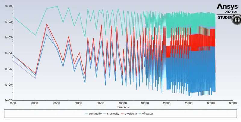
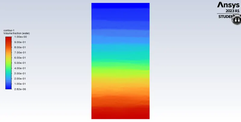
• Case 2: Base line mesh of 0.2mm.
  • Number of nodes is 20301.
  • The number of elements is 20000.
    
    
    
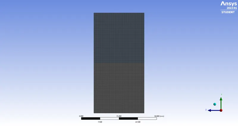
  • Scaled Residuals
    
    
    
  • Contours of volume fraction
    
    
    
    
  • Video link
    https://youtu.be/YtBu_cALvTY
    
    
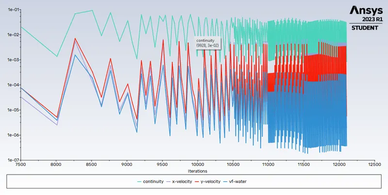
• Case 3: Mesh size is 0.2mm for water and user defined fluid.
  • Number of nodes is 20301.
  • The number of elements is 20000.
    
    
  • Scaled Residuals
    
    
    
  • Contours of volume fraction
    
    
    
  • Video Link
    https://youtu.be/h0nK-rOyYdY
    
    

Atwood Number
The Atwood number (A) is dimensionless in fluid dynamics used in the study of hydrodynamic instabilities in density stratified flows. It is a dimensionless density ratio defined as

`A=(rho1-rho2)/(rho1+rho2)`

where,
`rho1` = density of heavier fluid.
`rho2` = = density of lighter fluid.

In Rayleigh–Taylor instability, the penetration distance of heavy fluid bubbles into the lighter fluid is a function of the acceleration time scale, `Ag t^2`.

Where,
`g` = Gravitational Acceleration.
`t` = Time.

`rho` = 996
`rho`= 1.225

`A= (996-1.225)/(996+1.225)`

`A =1.02848`

Reason for choosing Transient state instead of steady state approach:
In Rayleigh Taylor Instability simulation, we are interested in observing the flow pattern and phase change behavior of the two fluids at every time step. So transient simulation is chosen in which the phase change is time bound behavior whereas in Steady state simulation is time independent study. We need to observe the mixing pattern at each stage in which the transient simulation is suitable.

Steady state simulation is carried only when we are interested in the end result only and the mixing of fluid behavior is not necessary. But here, the simulation time will be less.

Conclusion

• It is observed from the above experiment that when the mesh gets finer, the mixing pattern and phase change are clearly observed at each iteration and time step.
• As the mesh size gets finer, the simulation time gets increased since more cells are there to perform simulation. So it is necessary to choose optimum mesh size.
• Since the simulation involves capturing instabilities that are changing in an unpredictable manner as a function of time, the transient approach is preferred over the steady-state approach.
• For Atwood numbers close to 0, RT instability flows take the form of symmetric fingers of fluid.
• When Atwood number close to 1, the much lighter fluid below the heavier fluid takes the form of larger bubble-like plumes.