Week 5 - Rayleigh Taylor Instability

Answer:

Aim:

To perform simulation on mixing of two immiscible fluid under the effect of gravity and Simulate Rayleigh Taylor Instability Waves .

Objective:

1-To explain some practical CFD models that have been based on the mathematical analysis of Rayleigh Taylor waves.

2-To create geometry to perform simulation.

3-To perform the Rayleigh Taylor instability simulation on mesh size 0.5mm and take fluid material as water and air.

4-To perform the Rayleigh Taylor instability simulation on mesh size 0.3mm and take fluid material as water and air.

5-To compare the results by showing the animations

6-To explain the effect of mesh size on simulation

7-To explain why a steady-state approach might not be suitable for these types of simulation.

8-To perform the Rayleigh Taylor instability simulation on mesh size 0.3mm and take fluid material as water and and user-defined material(density = 400 kg/m³, viscosity = 0.001 kg/m-s) .

9-To Define the Atwood Number.

10-To find out the Atwood number for both the cases.

11-To explain how the variation in Atwood number in the above two cases affects the behavior of the instability.

Theory:

Introduction:

Rayleigh Taylor instability:Rayleigh–Taylor instability is the instability of an interface between two fluids of different densities which occures when the lighter fluids is pushing the heavier fluid.

practical CFD models that have been based on the mathematical analysis of Rayleigh Taylor waves:

1. KelvinHelmholtz instability -When two fluids of different velocity flow over each other then at their interface a shear velocity induces and this causes a shear stress .When this induced shear stress increased over the interface surface tension then disturbances at the iterface happens .This motion causes the appearance of a series of overturning ocean waves, a characteristic of the Kelvin–Helmholtz instabilit

2. Richtmyer Meshkov instability occurs when two fluids of different densities are impulsively accelerated. The penetration distance of heavy fluid bubbles into the lighter fluid is a function of the acceleration time scale. The development of the instability begins with small amplitude perturbations that initially grow linearly with time. This is followed by a nonlinear regime with bubbles appearing in the case of a light fluid penetrating a light fluid. A chaotic regime eventually is reached and the two fluids mix.

3. Rayleigh Plateauinstability.This type of instability occurs when a falling stream of fluid breaks up into smaller packets with the same volume bt less surface area. It is related to RT instability and part of a greater branch of fluid dynamics concerned with fluid thread breakup. This fluid instability is exploited in the design of a particular type of injector technology where a jet of liquid is perturbed into a steady stream of droplets. The driving force of the plateau rayleigh instability is that liquids, by virtue of their surface tensions tend to minimize their surface area.

4-Rayleigh Benard thermal convection-This type of instability occur when fluid layer flow between two plates at two different temperature because of which liquid layer in contact of hotter plate become less dense that the fluid near cooler plate and this create a convection current because of which instability happens.Since there is a density gradient between the top and the bottom plate, gravity acts trying to pull the cooler, denser liquid from the top to the bottom. This gravitational force is opposed by the viscous damping force in the fluid.

Geometry:

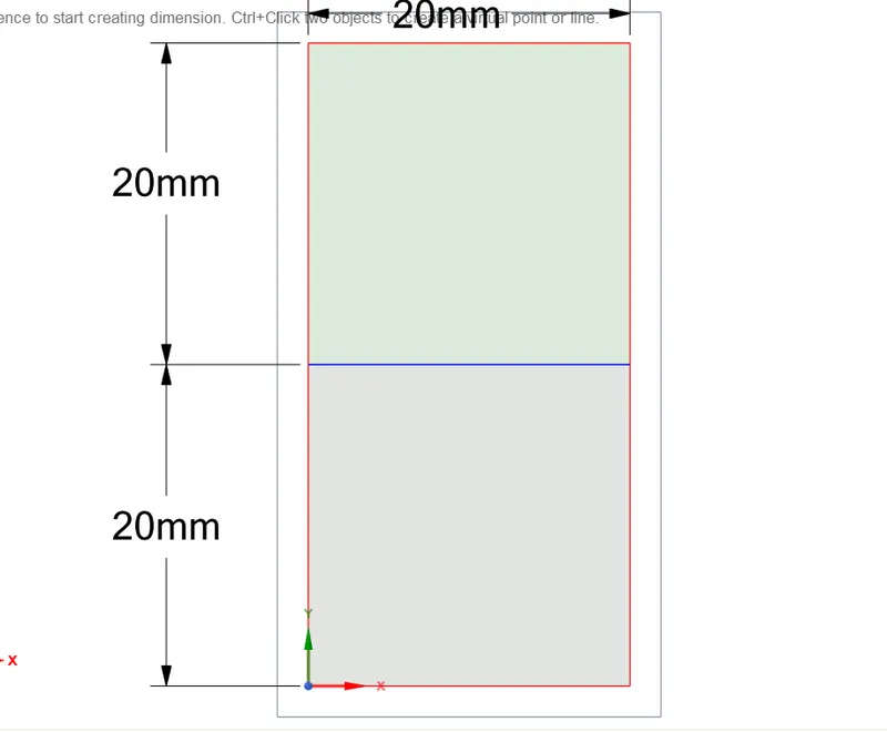
-Above geometry is created in space claim.

-Two component named as air(bottom one) and water(top one ) is created.

-Using PULL tool gemetry is converted into surface and share topology is enabled in Workbench.

Case1:

when whesh element size is equal to 0.5mm

Mesh:

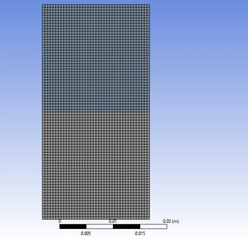
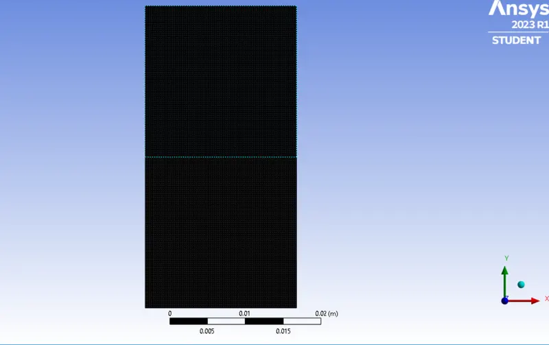
-Mesh element size is taken as 0.5mm

Solution and Results:

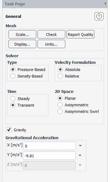
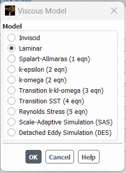
Solver and Setup:

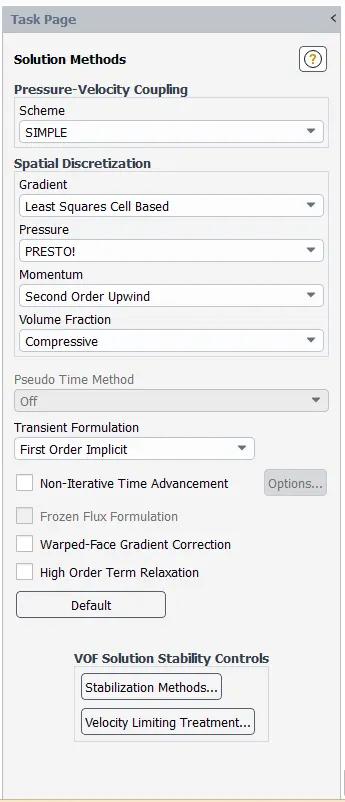
Multiphase:

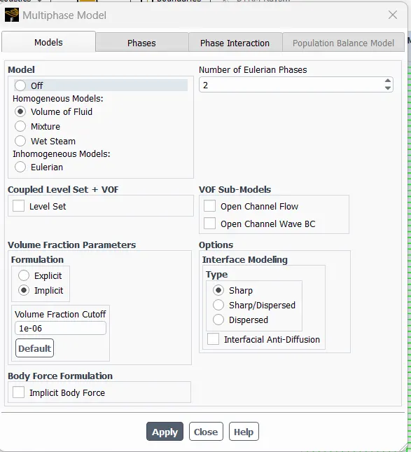
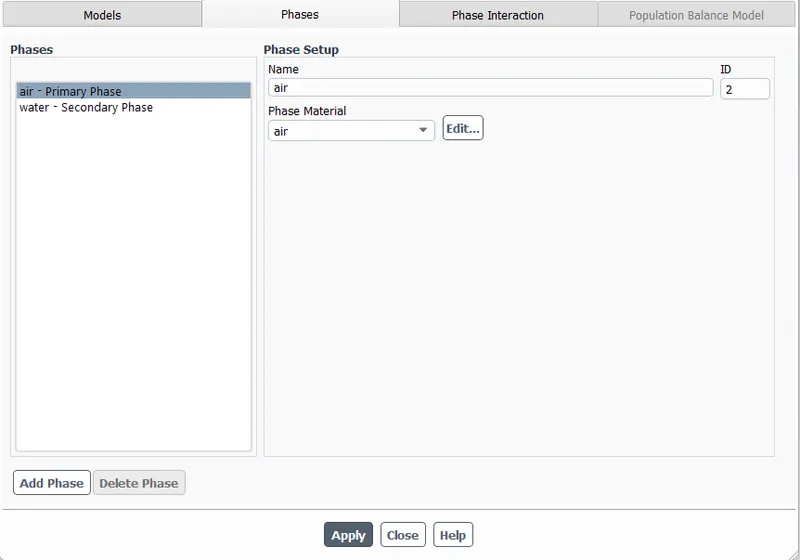
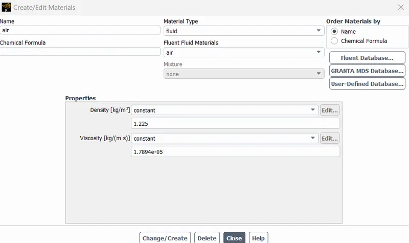
Materilas:

Two material Air and Liquid Water has been taken.

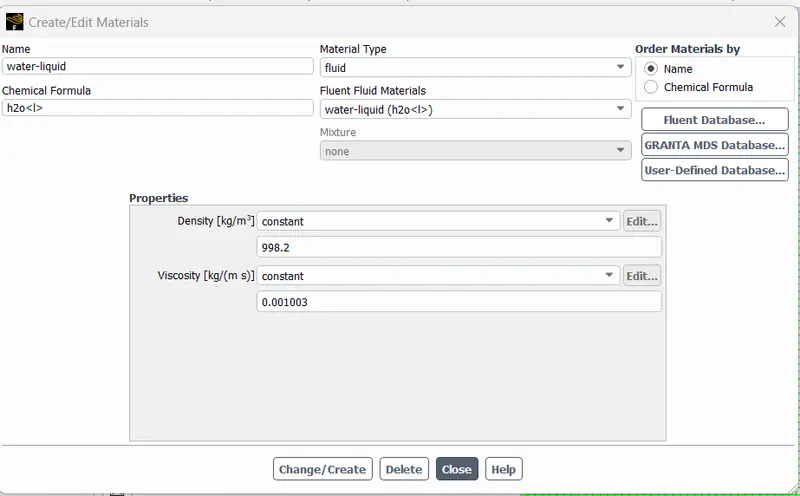
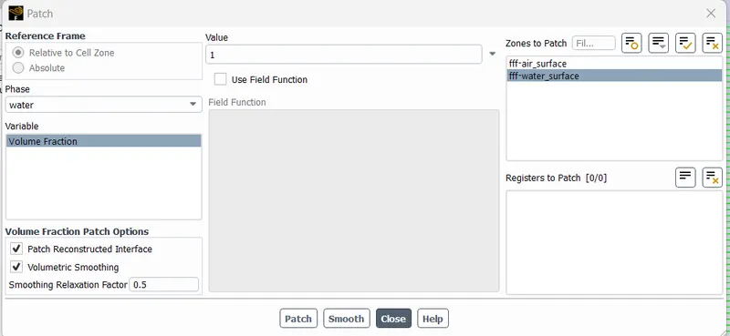
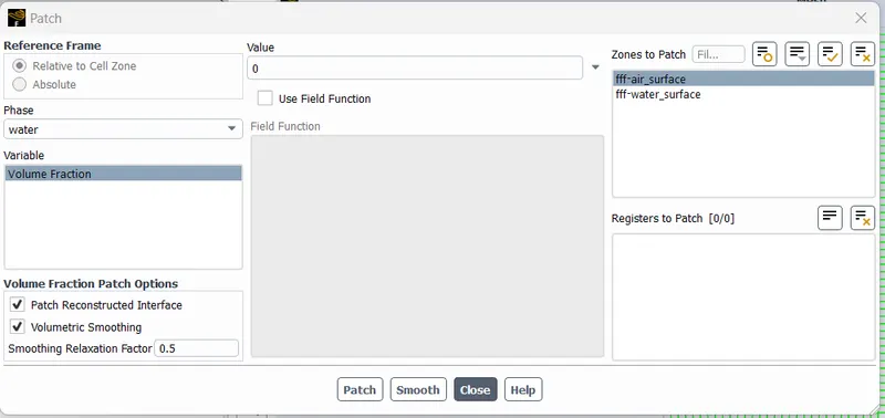
Patch:

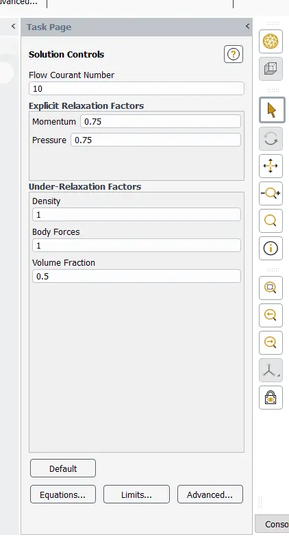
Solution Control:

Results:

Scale Residuals:

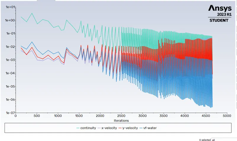
Contour:

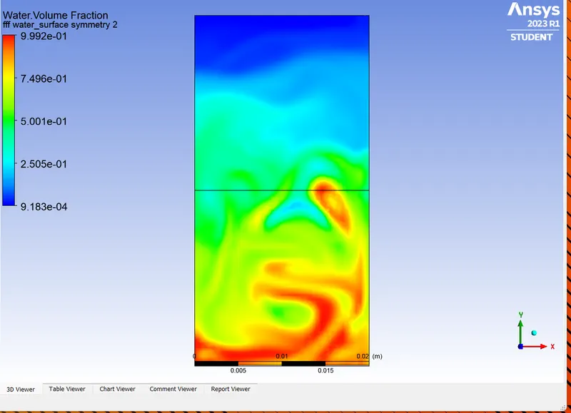
Animation Video Link:

https://drive.google.com/file/d/1BJGxuiVDamtM6E10_WKxk1bw4qLrwxZI/view?usp=sharing

Case2:

When mesh size is 0.3mm

Results:

Scale Residuals:

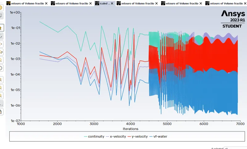
Animation File is attached here

https://drive.google.com/file/d/1XOXaG8KnZJm_XD8ODUGjIZUNB7OuWlta/view?usp=sharing

Effect of mesh size on simulation:

There is only effect of mesh size is better capture of motion of both fluids interface while moving to finally settle in equilibrium.

Why a steady-state approach might not be suitable for these types of simulation:

This phenominon is evolving with time .Each fluids interface is taking a specific turn at every moment annd variation in properties are time dependent.It following a path before settling down to equilibrium condidition hence to visualise the course of motion and change in behaviour transient simulation is needed.Otherwise there is no change in end results whether steady state simulation or trasient simulation is done

Case3:

When material iused idwater and user-defined material(density = 400 kg/m³, viscosity = 0.001 kg/m-s) for refined mesh.

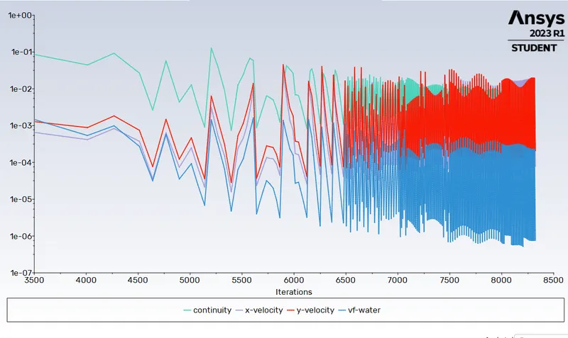
Scale Residuals:

Animation video link:

https://drive.google.com/file/d/1TiS_iqIy21Yo7j5zlnVEa6lD9PfkCJqq/view?usp=sharing

Atwood Number :

Atwood number equals the ratio of the difference in mass densities to their sum.It is a dimensionless number in fluid dynamics and it is used in the study of hydrodynamic instabilities in density-stratified flows.

Atwood number is an important parameter in the study of Rayleigh–Taylor instability and Richtmyer–Meshkov instability.

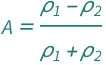
symbol	description	physical quantity
A	Atwood number	"AtwoodNumber"
ρ1	fluid density	"MassDensity"
ρ2	fluid density of lighter fluid	"MassDensity"

Atwood number for Case1:

ρ_{1(water)=998.2 kg/m^3}

_{ρ2(air)=1.225 kg/m^3}

_A=0.9975

_{Atwood number for Case3:}

ρ_{1(water)=998.2 kg/m^3}

_{ρ2(user_defined)=400 kg/m^3}

_A=0.427

_{Conclusion-At lower Atwood number it is taking more time to reach at quilibrium condition.When lighter fluid has comparitively lesser density as in Case 1 then faster mixing is happening resulting to faster reaching at equilibrium.}