Week 5 - Rayleigh Taylor Instability
AIM:
To run simulation and understand Rayleigh Taylor Instability.
OBJECTIVE:
- Discussion on practical CFD models that have been based on the mathematical analysis of Rayleigh Taylor waves. Explanation of these mathematical models on its adaptation for CFD calculations
- Perform the Rayleigh Taylor instability simulation for 2 different mesh sizes with the base mesh being 0.5 mm and refined mesh being 0.2 and observe the variations of these instabilities in Ansys fluent and explanation on the reason behind viability of transient approach instead of steady state approach.
- Run one more simulation with water and user-defined material(density = 400 kg/m3, viscosity = 0.001 kg/m-s) for refined mesh.
- Define the Atwood Number. Find out the Atwood number for both the cases and explanation of the variation in Atwood number in the above two cases and it’s effects on the behaviour of the instability.
INTRODUCTION:
Rayleigh Taylor instability is an instability of the interface separating two immiscible fluids., the densest of which rests on the lightest. Following a disturbance of the interface, the dense fluid enters the light fluid. This simulation is run on a 2D frame and captured in animation in this project. For different mesh sizes and different densities of fluids flow patterns will be captured. Variation of atwood number will be verified in this project. Transient state analysis is done to see how the interface collapses as the function of time.
THEORY:
Rayleigh Taylor Instability
The RT Instability is the instability that occurs at the interface of two fluids of different densities. The lower density fluid pushes the higher density fluid. Examples are oil pushing water when water is at top due to gravity forces. Mushroom clouds due to volcanic eruptions are examples of RT Instability.
When water is lying above a oil on a parallel surface. The potential energy of denser fluid is higher. As the water displaces equal volume of oil from its position and disturbance increases there is release of potential energy. This setup was studied by Lord Rayleigh. Taylor noted that as acceleration of these fluid particles increases more fluid pushes denser fluid from its position.
As RT instability develops the initial perturbations increase from a linear to non linear form. It starts developing in the form of plumes in upward direction with spikes pointing towards the downward directions. In the linear phase perturbations was accounted to be in the amplitude variations in exponential manner but as flow progressed amplitude was so high than to be realised by linear equations to change ethe order to non-linearity. This density disparity determines the structure of non linearity. And this density disparity is given by Atwood number A.
A=(Density of heavier fluid – Density of lighter fluid)/ (Density of heavier fluid + Density of lighter fluid).
If A = 0, RT instability will be of the form symmetric fingers and if A =1 , RT instability will be of the form bubble like plumes.
Kelvin-Helmholtz Instability
The Kelvin–Helmholtz instability (after Lord Kelvin and Hermann von Helmholtz) is a fluid instability that occurs when there is velocity shear in a single continuous fluid or a velocity difference across the interface between two fluids. Kelvin-Helmholtz instabilities are visible in the atmospheres of planets and moons, such as in cloud formations on Earth or the Red Spot on Jupiter, and the atmospheres of the Sun and other stars
Fluid dynamics predicts the onset of instability and transition to turbulent flow within fluids of different densities moving at different speeds. If surface tension is ignored, two fluids in parallel motion with different velocities and densities yield an interface that is unstable to short-wavelength perturbations for all speeds. However, surface tension is able to stabilize the short wavelength instability up to a threshold velocity.
Richtmyer-Meshkov Instability
The Richtmyer–Meshkov instability (RMI) occurs when two fluids of different density are impulsively accelerated. Normally this is by the passage of a shock wave. The development of the instability begins with small amplitude perturbations which initially grow linearly with time. This is followed by a nonlinear regime with bubbles appearing in the case of a light fluid penetrating a heavy fluid, and with spikes appearing in the case of a heavy fluid penetrating a light fluid. A chaotic regime eventually is reached and the two fluids mix. This instability can be considered the impulsive-acceleration limit of the Rayleigh–Taylor instability.
Plateau-Rayleigh Instability
The Plateau–Rayleigh instability, often just called the Rayleigh instability, explains why and how a falling stream of fluid breaks up into smaller packets with the same volume but less surface area. It is related to the Rayleigh–Taylor instability and is part of a greater branch of fluid dynamics concerned with fluid thread breakup. This fluid instability is exploited in the design of a particular type of ink jet technology whereby a jet of liquid is perturbed into a steady stream of droplets.
The driving force of the Plateau–Rayleigh instability is that liquids, by virtue of their surface tensions, tend to minimize their surface area. A considerable amount of work has been done recently on the final pinching profile by attacking it with self-similar solutions.
PROCEDURE:
SOLVING AND MODELLING APPROACH:
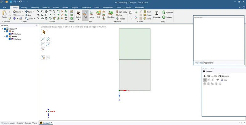
- Geometry is made in spaceclaim
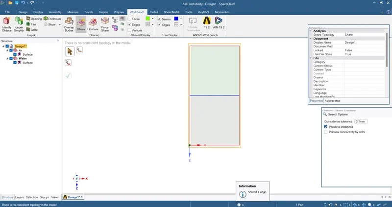
- For creating conformal mesh. Air and water surfaces are shared at interface
PREPROCESSING AND SOLVER SETTING:
MESH SETTING:
- Open the mesh
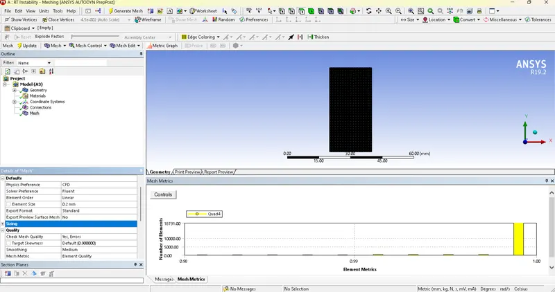
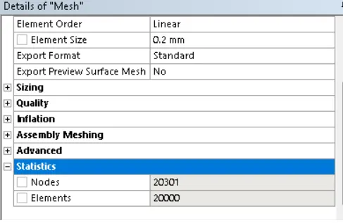
- Run baseline mesh with 0.5 mm mesh length
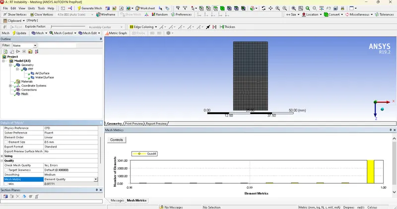
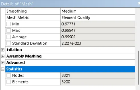
- After 1st round simulation Run refined mesh length of 0.2mm.
SOLVER SETTING (Air-Water Interface(for 0.5 mm mesh and 0.2 mm mesh):
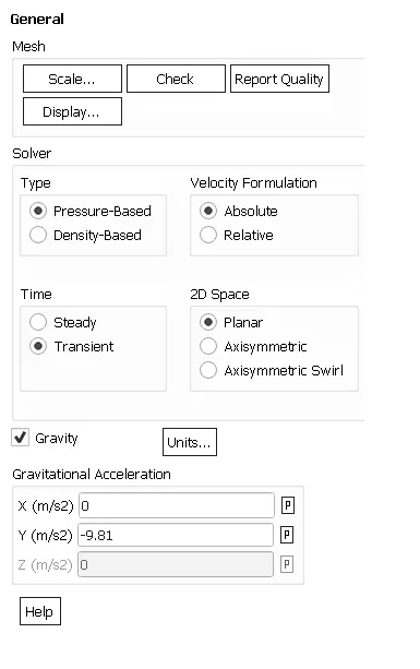
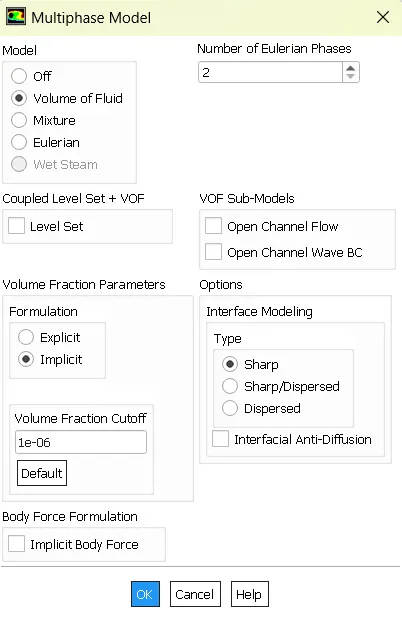
- Model:Pressure based – transient state flow, Viscous -Laminar selected, MultiPhase-Volume of fluid selected with implicit scheme.
- Materials= Air, water with default settings.
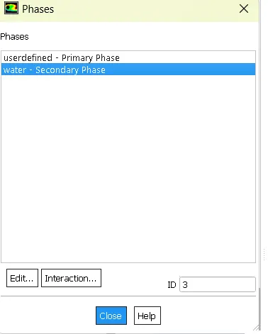
- Phases selected as water and air as secondary and primary phases.
- Standard Initialize with time step 0.005 and no: of time steps 1500.
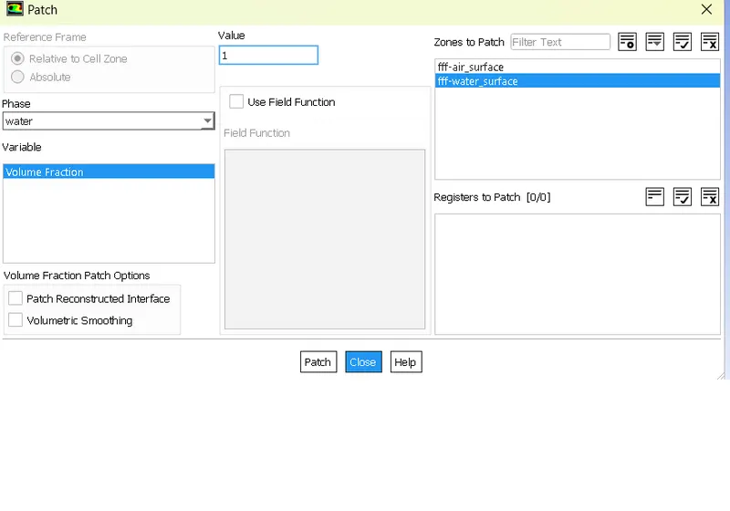
- Now select patch and set water volume of fraction as 1 for water surface and set water is 0 for air surface.
- Select phase contour from post processing and create animation pane.
- Run Calculation.
SOLVER SETTING (User defined fluid-Water Interface) (for 0.2 mm mesh):
- Model:Pressure based – transient state flow, Viscous -Laminar selected, MultiPhase-Volume of fluid selected with implicit scheme.
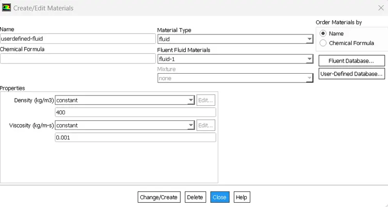
- Materials= User defined fluid with density 400 kg/m3 and viscosity 001 kg/m-s , water with default settings.
- Phases selected as water and user defined fluid as secondary and primary phases.
- Standard Initialize with time step 0.005 and no: of time steps 1500.
- Now select patch and set water volume of fraction as 1 for water surface and set water is 0 for air surface.
- Select phase contour from post processing and create animation pane.
- Run Calculation.
POST PROCESSING
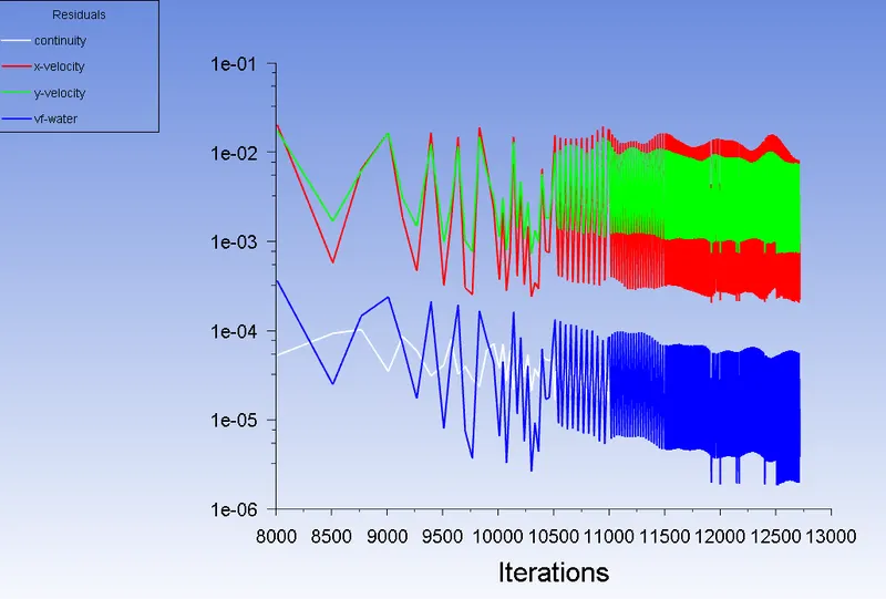
Residuals plotted for checking convergence and video written in mpeg format for each cases.
RESULT:
CASE:1 0.5mm mesh Air – Water Interface
Transient state residuals and video animation attached.
Animation Link of 0.5 mm baseline mesh Rayleigh Taylor Instability of Air-Water Interface:
https://drive.google.com/file/d/1KmLCDO4gbaBqisRmqqRBmTV7bvDAIoV_/view?usp=sharing
CASE:1 0.2mm mesh Air – Water Interface
Transient state residuals and video animation attached.
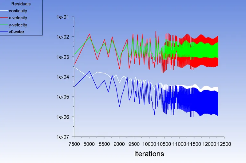
Animation Link of 0.2 mm baseline mesh Rayleigh Taylor Instability of Air-Water Interface:
https://drive.google.com/file/d/1_Q4U9jQ5r4GM987oEZZTgwr6pasb-g_N/view?usp=sharing
CASE:1 0.2mm mesh User defined fluid – Water Interface
Transient state residuals and video animation attached.
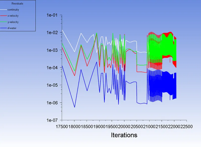
Animation Link of 0.2 mm baseline mesh Rayleigh Taylor Instability of UserDefined fluid-Water Interface:
https://drive.google.com/file/d/1x5rRTtrgED_XVUnAAnb_OwmbMhRz2-52/view?usp=sharing
CONCLUSION:
The steady state calculations are useful when the study is focused on to calculate or simulate the end results. Here in this study, the instabilities information is sensitive and completely time-dependent. At each and every time step, the instabilities grow exponentially. Though steady state simulation is capable to capture those instabilities but the results would not be time-accurate. Anyways transient state calculation with reduced time-steps can capture these instabilities at each and every time-steps and sensible time dependent results can be obtained.
Atwood Number:
It is a dimensionless number in fluid dynamics used in the study of hydrodynamic instabilities in density stratified flows. It is a dimensionless density ratio defined as
Atwood number(A)=(Density of heavier fluid – Density of lighter fluid)/ (Density of heavier fluid + Density of lighter fluid).
If A = 0, RT instability will be of the form symmetric fingers and if A =1 , RT instability will be of the form bubble like plumes.
Atwood number for Air-Water Interface
A=(Density of heavier fluid – Density of lighter fluid)/ (Density of heavier fluid + Density of lighter fluid).
A=(998.2– 1.225)/ (998.2 + 1.225) = 0.9975
Atwood number for User defined fluid-Water Interface
A=(Density of heavier fluid – Density of lighter fluid)/ (Density of heavier fluid + Density of lighter fluid).
A=(998.2– 400)/ (998.2 + 400) = 0.4278
It was noted from the animation panes attached for air water interface and user defined fluid and water interface that latter one had symmetric finger like shapes but former one had more bubble like plumes with downward spikes. So it is clear that Simulation gave better results and is in conformal with Atwood number.
REFERENCES: