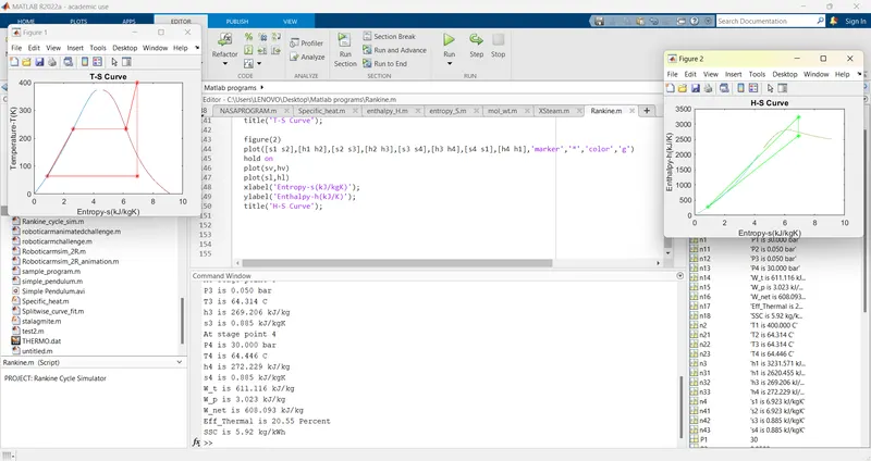
Project 2 - Rankine cycle Simulator
AIM:
To create a program code to run Rankine Cycle Simulator.
SOFTWARE USED:
Matlab
GOVERNING EQUATIONS:
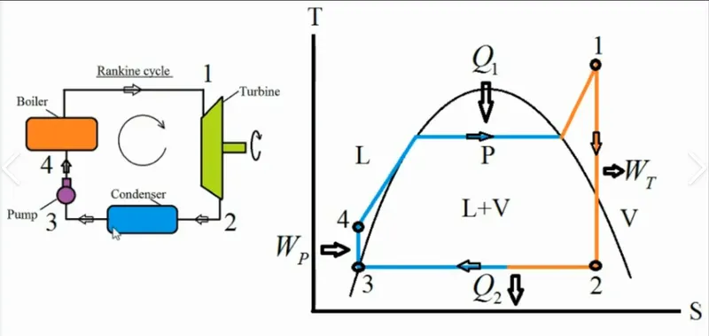
1-2 is Isentropic Expansion in the Turbine
2-3 is Constant Pressure Heat Rejection by the Condensor
3-4 is Isentropic Expansion in the Pump
4-1 is Constant Pressure Heat Addition to the Boiler
OBJECTIVES:
- Create a Rankine Cycle Simulator using MATLAB.
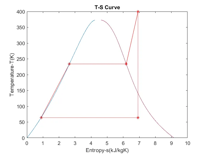
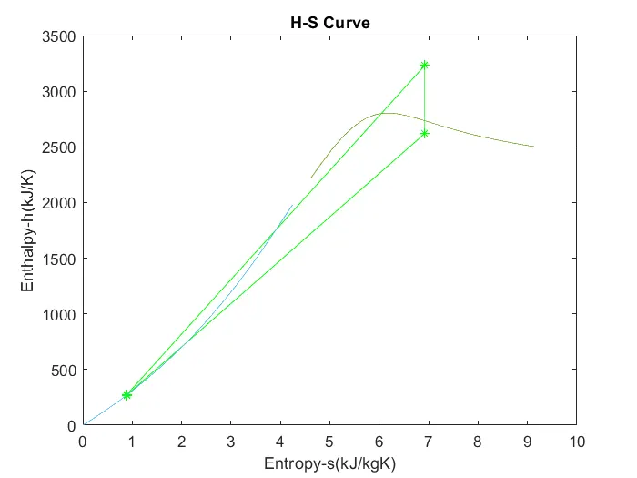
- Plot the corresponding T-s and h-s plots for the given set of inputs.
Required Inputs:
Turbine Inlet temperature = 400° C
Turbine Inlet Pressure = 30 bars
Turbine Outlet Pressure = 0.05 bars = Condenser Inlet Pressure
BODY OF CONTEXT:
% PROJECT: Rankine Cycle Simulator
clear all; % clear all variables in workspace
close all;% close all plots
clc;%clear command window
disp(' RANKINE CYCLE SIMULATOR');
disp('1-2 is Isentropic Expansion in the Turbine');
disp('2-3 is Constant Pressure Heat Rejection by the Condensor');
disp('3-4 is Isentropic Expansion in the Pump');
disp('4-1 is Constant Pressure Heat Addition to the Boiler');
%Inputs
disp('INPUTS');
P1=input('Enter the Pressure at turbine inlet(bar):');
T1=input('Enter the Temperature at the Turbine inlet(degree C):');
P2=input('Enter the Pressure at the Condensor(bar):');
%Using the Xsteam functions, enthalpy and entropy at various points can be
%calculated
%Calculating enthalpy(h) and entropy(s) at point 1:
h1=XSteam('h_pT',P1,T1);
s1=XSteam('s_pT',P1,T1);
%Calculating pressure(P),enthalpy(h) and entropy(s) at point 2
%Since isentropic expansion
s2=s1;
%For isentropic expansion, (T2/T1)=(P2/P1)^(1-(1/g))
g=1.4;
power=1-(1/g);
T2=T1*((P2/P1)^power);
h2=XSteam('h_pT',P2,T2);
%Calculating pressure, enthalpy and entropy at point 2
%Since constant pressure heat removal
P3=P2;
T3=T2;
h3=XSteam('hL_T',T3);
s3=XSteam('sL_T',T3);
%Calculating pressure, enthalpy and entropy at point 4
%Since isentropic compression
s4=s3;
%Since constant pressure proces
P4=P1;
T4=XSteam('T_ps',P4,s4);
h4=XSteam('h_pT',P4,T4);
h41=XSteam('hL_p',P4);
s41=XSteam('sL_p',P4);
h42=XSteam('hV_p',P4);
s42=XSteam('sV_p',P4);
T41=XSteam('T_hs',h41,s41);
T42=XSteam('T_hs',h42,s42);
%Calculating entropy and enthalpy at the saturation curve
Temp=linspace(0,500,600);
for i=1:length(Temp)
sv(i)=XSteam('sV_T',Temp(i));
sl(i)=XSteam('sL_T',Temp(i));
hv(i)=XSteam('hV_T',Temp(i));
hl(i)=XSteam('hL_T',Temp(i));
end
%Calculating the net work output (W_net)
W_t=h1-h2;
W_p=h4-h3;
W_net=W_t-W_p;
%Calculating back work ratio
Bw_ratio=W_p/W_t;
%Calculating thermal efficiency
Q_in=h1-h4;
eff_thermal=(W_net/Q_in)*100;
%Calculating specific steam consumption, 1J=3600 kg/s
SSC=3600/W_net;
%Displaying results in the command window
disp(' RESULTS');
P1=P1;
T1=T1;
P2=P2;
disp('At stage point 1');
n1=sprintf('P1 is %.3f bar',P1);
disp(n1);
n2=sprintf('T1 is %.3f C',T1);
disp(n2);
n3=sprintf('h1 is %.3f kJ/kg',h1);
disp(n3);
n4=sprintf('s1 is %.3f kJ/kgK',s1);
disp(n4);
disp('At stage point 2');
n11=sprintf('P2 is %.3f bar',P2);
disp(n11);
n21=sprintf('T2 is %.3f C',T2);
disp(n21);
n31=sprintf('h1 is %.3f kJ/kg',h2);
disp(n31);
n41=sprintf('s2 is %.3f kJ/kgK',s2);
disp(n41);
disp('At stage point 3');
n12=sprintf('P3 is %.3f bar',P3);
disp(n12);
n22=sprintf('T3 is %.3f C',T3);
disp(n22);
n32=sprintf('h3 is %.3f kJ/kg',h3);
disp(n32);
n42=sprintf('s3 is %.3f kJ/kgK',s3);
disp(n42);
disp('At stage point 4');
n13=sprintf('P4 is %.3f bar',P4);
disp(n13);
n23=sprintf('T4 is %.3f C',T4);
disp(n23);
n33=sprintf('h4 is %.3f kJ/kg',h4);
disp(n33);
n43=sprintf('s4 is %.3f kJ/kgK',s4);
disp(n43);
n14=sprintf('W_t is %.3f kJ/kg',W_t);
disp(n14);
n15=sprintf('W_p is %.3f kJ/kg',W_p);
disp(n15);
n16=sprintf('W_net is %.3f kJ/kg',W_net);
disp(n16);
n17=sprintf('Eff_Thermal is %.2f Percent',eff_thermal);
disp(n17);
n18=sprintf('SSC is %.2f kg/kWh',SSC);
disp(n18);
figure(1)
plot([s1 s2],[T1 T2],[s2 s3],[T2 T3],[s3 s4],[T3 T4],[s4 s41],[T4 T41],[s41 s42],[T41 T42],[s42 s1],[T42 T1],'marker','*','color','r')
hold on
plot(sv,Temp)
plot(sl,Temp)
xlabel('Entropy-s(kJ/kgK)');
ylabel('Temperature-T(K)');
title('T-S Curve');
figure(2)
plot([s1 s2],[h1 h2],[s2 s3],[h2 h3],[s3 s4],[h3 h4],[s4 s1],[h4 h1],'marker','*','color','g')
hold on
plot(sv,hv)
plot(sl,hl)
xlabel('Entropy-s(kJ/kgK)');
ylabel('Enthalpy-h(kJ/K)');
title('H-S Curve');
PROGRAM CODE:
% PROJECT: Rankine Cycle Simulator
clear all; % clear all variables in workspace
close all;% close all plots
clc;%clear command window
disp('                             RANKINE CYCLE SIMULATOR');
disp('1-2 is Isentropic Expansion in the Turbine');
disp('2-3 is Constant Pressure Heat Rejection by the Condensor');
disp('3-4 is Isentropic Expansion in the Pump');
disp('4-1 is Constant Pressure Heat Addition to the Boiler');

%Inputs
disp('INPUTS');
P1=input('Enter the Pressure at turbine inlet(bar):');
T1=input('Enter the Temperature at the Turbine inlet(degree C):');
P2=input('Enter the Pressure at the Condensor(bar):');

%Using the Xsteam functions, enthalpy and entropy at various points can be
%calculated

%Calculating enthalpy(h) and entropy(s) at point 1:
h1=XSteam('h_pT',P1,T1);
s1=XSteam('s_pT',P1,T1);

%Calculating pressure(P),enthalpy(h) and entropy(s) at point 2
%Since isentropic expansion
s2=s1;

%For isentropic expansion, (T2/T1)=(P2/P1)^(1-(1/g))
g=1.4;
power=1-(1/g);
T2=T1*((P2/P1)^power);
h2=XSteam('h_pT',P2,T2);

%Calculating pressure, enthalpy and entropy at point 2
%Since constant pressure heat removal
P3=P2;
T3=T2;
h3=XSteam('hL_T',T3);
s3=XSteam('sL_T',T3);

%Calculating pressure, enthalpy and entropy at point 4
%Since isentropic compression
s4=s3;

%Since constant pressure proces
P4=P1;
T4=XSteam('T_ps',P4,s4);
h4=XSteam('h_pT',P4,T4);
h41=XSteam('hL_p',P4);
s41=XSteam('sL_p',P4);
h42=XSteam('hV_p',P4);
s42=XSteam('sV_p',P4);
T41=XSteam('T_hs',h41,s41);
T42=XSteam('T_hs',h42,s42);

%Calculating entropy and enthalpy at the saturation curve
Temp=linspace(0,500,600);
for i=1:length(Temp)
    sv(i)=XSteam('sV_T',Temp(i));
    sl(i)=XSteam('sL_T',Temp(i));

    hv(i)=XSteam('hV_T',Temp(i));
    hl(i)=XSteam('hL_T',Temp(i));
end

%Calculating the net work output (W_net)
W_t=h1-h2;
W_p=h4-h3;
W_net=W_t-W_p;

%Calculating back work ratio
Bw_ratio=W_p/W_t;

%Calculating thermal efficiency
Q_in=h1-h4;
eff_thermal=(W_net/Q_in)*100;

%Calculating sepcific steam consumption, 1J=3600 kg/s
SSC=3600/W_net;

%Displaying results in the command window
disp('                             RESULTS');
P1=P1;
T1=T1;
P2=P2;
disp('At stage point 1');
n1=sprintf('P1 is %.3f bar',P1);
disp(n1);
n2=sprintf('T1 is %.3f C',T1);
disp(n2);
n3=sprintf('h1 is %.3f kJ/kg',h1);
disp(n3);
n4=sprintf('s1 is %.3f kJ/kgK',s1);
disp(n4);
disp('At stage point 2');
n11=sprintf('P2 is %.3f bar',P2);
disp(n11);
n21=sprintf('T2 is %.3f C',T2);
disp(n21);
n31=sprintf('h1 is %.3f kJ/kg',h2);
disp(n31);
n41=sprintf('s2 is %.3f kJ/kgK',s2);
disp(n41);
disp('At stage point 3');
n12=sprintf('P3 is %.3f bar',P3);
disp(n12);
n22=sprintf('T3 is %.3f C',T3);
disp(n22);
n32=sprintf('h3 is %.3f kJ/kg',h3);
disp(n32);
n42=sprintf('s3 is %.3f kJ/kgK',s3);
disp(n42);
disp('At stage point 4');
n13=sprintf('P4 is %.3f bar',P4);
disp(n13);
n23=sprintf('T4 is %.3f C',T4);
disp(n23);
n33=sprintf('h4 is %.3f kJ/kg',h4);
disp(n33);
n43=sprintf('s4 is %.3f kJ/kgK',s4);
disp(n43);
n14=sprintf('W_t is %.3f kJ/kg',W_t);
disp(n14);
n15=sprintf('W_p is %.3f kJ/kg',W_p);
disp(n15);
n16=sprintf('W_net is %.3f kJ/kg',W_net);
disp(n16);
n17=sprintf('Eff_Thermal is %.2f Percent',eff_thermal);
disp(n17);
n18=sprintf('SSC is %.2f kg/kWh',SSC);
disp(n18);


figure(1)
plot([s1 s2],[T1 T2],[s2 s3],[T2 T3],[s3 s4],[T3 T4],[s4 s41],[T4 T41],[s41 s42],[T41 T42],[s42 s1],[T42 T1],'marker','*','color','r')
hold on
plot(sv,Temp)
plot(sl,Temp)
xlabel('Entropy-s(kJ/kgK)');
ylabel('Temperature-T(K)');
title('T-S Curve');

figure(2)
plot([s1 s2],[h1 h2],[s2 s3],[h2 h3],[s3 s4],[h3 h4],[s4 s1],[h4 h1],'marker','*','color','g')
hold on
plot(sv,hv)
plot(sl,hl)
xlabel('Entropy-s(kJ/kgK)');
ylabel('Enthalpy-h(kJ/K)');
title('H-S Curve');
SYNTAX FOR PROGRAM WITH EXPLANATION:
disp(' RANKINE CYCLE SIMULATOR');
disp('1-2 is Isentropic Expansion in the Turbine');
disp('2-3 is Constant Pressure Heat Rejection by the Condensor');
disp('3-4 is Isentropic Expansion in the Pump');
disp('4-1 is Constant Pressure Heat Addition to the Boiler');
<--Inputs
disp('INPUTS');
P1=input('Enter the Pressure at turbine inlet(bar):');
T1=input('Enter the Temperature at the Turbine inlet(degree C):');
P2=input('Enter the Pressure at the Condensor(bar):');
<--Using the Xsteam functions, enthalpy and entropy at various points can be
<--calculated
<--Calculating enthalpy(h) and entropy(s) at point 1:
h1=XSteam('h_pT',P1,T1);
s1=XSteam('s_pT',P1,T1);
<--Calculating pressure(P),enthalpy(h) and entropy(s) at point 2
<--Since isentropic expansion
s2=s1;
<--For isentropic expansion, (T2/T1)=(P2/P1)^(1-(1/g))
g=1.4;
power=1-(1/g);
T2=T1*((P2/P1)^power);
h2=XSteam('h_pT',P2,T2);
<--Calculating pressure, enthalpy and entropy at point 2
<--Since constant pressure heat removal
P3=P2;
T3=T2;
h3=XSteam('hL_T',T3);
s3=XSteam('sL_T',T3);
<--Calculating pressure, enthalpy and entropy at point 4
<--Since isentropic compression
s4=s3;
<--Since constant pressure proces
P4=P1;
T4=XSteam('T_ps',P4,s4);
h4=XSteam('h_pT',P4,T4);
h41=XSteam('hL_p',P4);
s41=XSteam('sL_p',P4);
h42=XSteam('hV_p',P4);
s42=XSteam('sV_p',P4);
T41=XSteam('T_hs',h41,s41);
T42=XSteam('T_hs',h42,s42);
<--Calculating entropy and enthalpy at the saturation curve
Temp=linspace(0,500,600);
for i=1:length(Temp)
sv(i)=XSteam('sV_T',Temp(i));
sl(i)=XSteam('sL_T',Temp(i));
hv(i)=XSteam('hV_T',Temp(i));
hl(i)=XSteam('hL_T',Temp(i));
end
<--Calculating the net work output (W_net)
W_t=h1-h2;
W_p=h4-h3;
W_net=W_t-W_p;
<--Calculating back work ratio
Bw_ratio=W_p/W_t;
<--Calculating thermal efficiency
Q_in=h1-h4;
eff_thermal=(W_net/Q_in)*100;
<--Calculating sepcific steam consumption, 1J=3600 kg/s
SSC=3600/W_net;
<--Displaying results in the command window
disp(' RESULTS');
P1=P1;
T1=T1;
P2=P2;
disp('At stage point 1');
n1=sprintf('P1 is <--.3f bar',P1);
disp(n1);
n2=sprintf('T1 is <--.3f C',T1);
disp(n2);
n3=sprintf('h1 is <--.3f kJ/kg',h1);
disp(n3);
n4=sprintf('s1 is <--.3f kJ/kgK',s1);
disp(n4);
disp('At stage point 2');
n11=sprintf('P2 is <--.3f bar',P2);
disp(n11);
n21=sprintf('T2 is <--.3f C',T2);
disp(n21);
n31=sprintf('h1 is <--.3f kJ/kg',h2);
disp(n31);
n41=sprintf('s2 is <--.3f kJ/kgK',s2);
disp(n41);
disp('At stage point 3');
n12=sprintf('P3 is <--.3f bar',P3);
disp(n12);
n22=sprintf('T3 is <--.3f C',T3);
disp(n22);
n32=sprintf('h3 is <--.3f kJ/kg',h3);
disp(n32);
n42=sprintf('s3 is <--.3f kJ/kgK',s3);
disp(n42);
disp('At stage point 4');
n13=sprintf('P4 is <--.3f bar',P4);
disp(n13);
n23=sprintf('T4 is <--.3f C',T4);
disp(n23);
n33=sprintf('h4 is <--.3f kJ/kg',h4);
disp(n33);
n43=sprintf('s4 is <--.3f kJ/kgK',s4);
disp(n43);
n14=sprintf('W_t is <--.3f kJ/kg',W_t);
disp(n14);
n15=sprintf('W_p is <--.3f kJ/kg',W_p);
disp(n15);
n16=sprintf('W_net is <--.3f kJ/kg',W_net);
disp(n16);
n17=sprintf('Eff_Thermal is <--.2f Percent',eff_thermal);
disp(n17);
n18=sprintf('SSC is <--.2f kg/kWh',SSC);
disp(n18);
figure(1)
plot([s1 s2],[T1 T2],[s2 s3],[T2 T3],[s3 s4],[T3 T4],[s4 s41],[T4 T41],[s41 s42],[T41 T42],[s42 s1],[T42 T1],'marker','*','color','r')
hold on
plot(sv,Temp)
plot(sl,Temp)
xlabel('Entropy-s(kJ/kgK)');
ylabel('Temperature-T(K)');
title('T-S Curve');
figure(2)
plot([s1 s2],[h1 h2],[s2 s3],[h2 h3],[s3 s4],[h3 h4],[s4 s1],[h4 h1],'marker','*','color','g')
hold on
plot(sv,hv)
plot(sl,hl)
xlabel('Entropy-s(kJ/kgK)');
ylabel('Enthalpy-h(kJ/K)');
title('H-S Curve');
CONCLUSION:
RANKINE CYCLE SIMULATOR
1-2 is Isentropic Expansion in the Turbine
2-3 is Constant Pressure Heat Rejection by the Condensor
3-4 is Isentropic Expansion in the Pump
4-1 is Constant Pressure Heat Addition to the Boiler
INPUTS
Enter the Pressure at turbine inlet(bar):30
Enter the Temperature at the Turbine inlet(degree C):400
Enter the Pressure at the Condensor(bar):0.05
RESULTS
At stage point 1
P1 is 30.000 bar
T1 is 400.000 C
h1 is 3231.571 kJ/kg
s1 is 6.923 kJ/kgK
At stage point 2
P2 is 0.050 bar
T2 is 64.314 C
h1 is 2620.455 kJ/kg
s2 is 6.923 kJ/kgK
At stage point 3
P3 is 0.050 bar
T3 is 64.314 C
h3 is 269.206 kJ/kg
s3 is 0.885 kJ/kgK
At stage point 4
P4 is 30.000 bar
T4 is 64.446 C
h4 is 272.229 kJ/kg
s4 is 0.885 kJ/kgK
W_t is 611.116 kJ/kg
W_p is 3.023 kJ/kg
W_net is 608.093 kJ/kg
Eff_Thermal is 20.55 Percent
SSC is 5.92 kg/kWh
>>