Week 5 - Rayleigh Taylor Instability

Aim:

• To study the concept of Rayleigh Taylor Instability and some practical CFD models that have been based on the mathematical analysis of Rayleigh Taylor waves.
• To study the Rayleigh Taylor Instability simulation for 2 different mesh sizes in addition to baseline and compare the results.
• To study the the effect of Atwood number variation on Rayleigh Taylor Instability for all the cases.

Objective:

1. What are some practical CFD models that have been based on the mathematical analysis of Rayleigh Taylor waves? In your own words, explain how these mathematical models have been adapted for CFD calculations.
2. Perform the Rayleigh Taylor instability simulation for 2 different mesh sizes with the base mesh being 0.5 mm. Compare the results by showing the animations( Attach them from your google drive). Observe the differences in the animation and explain the effect of mesh size on simulation. Also, explain why a steady-state approach might not be suitable for these types of simulation.[ Choose Air and Water for this simulation].
3. Run one more simulation with water and user-defined material(density = 400 kg/m³, viscosity = 0.001 kg/m-s) for refined mesh.
4. Define the Atwood Number. Find out the Atwood number for both the cases and explain how the variation in Atwood number in the above two cases affects the behavior of the instability.

1.

The Rayleigh–Taylor instability, or RT instability, is the instability of an interface between two fluids of different densities which occurs when the lighter fluid is pushing the heavier fluid. Examples include the behavior of water suspended above oil in the gravity of earth, mushroom clouds like those from a volcanic eruption and atmospheric nuclear explosion, supernova explosions in which expanding core gas is accelerated into denser shell gas, instabilities in plasma fusion reactors, and inertial confinement fusion.

Water suspended atop oil is an everyday example of Rayleigh–Taylor instability, and it may be modeled by two completely plane-parallel layers of immiscible fluid, the denser on top of the less dense one and both subject to the Earth's gravity. The equilibrium here is unstable to any perturbations or disturbances of the interface: if a parcel of heavier fluid is displaced downward with an equal volume of lighter fluid displaced upwards, the potential energy of the configuration is lower than the initial state. Thus the disturbance will grow and lead to a further release of potential energy, as the more dense material moves down under the (effective) gravitational field, and the less dense material is further displaced upwards. This was the set-up as studied by Lord Rayleigh. The important insight by G. I. Taylor was his realization that this situation is equivalent to the situation when the fluids are accelerated, with the less dense fluid accelerating into the more dense fluid. This occurs deep underwater on the surface of an expanding bubble and in a nuclear explosion

Types of Instability and some practical CFD models that have been based on the mathematical analysis of Rayleigh Taylor waves:

Ritchmyer-Meshkov instability:

The Richtmyer-Meshkov instability arises when a shock wave interacts with an interface separating two different fluids. It combines compressible phenomena, such as shock interaction and refraction, with hydrodynamic instability, including nonlinear growth and subsequent transition to turbulence, across a wide range of Mach numbers.

Plateau–Rayleigh instability:

The Plateau–Rayleigh instability, often just called the Rayleigh instability, explains why and how a falling stream of fluid breaks up into smaller packets with the same volume but less surface area. This fluid instability is exploited in the design of a particular type of inkjet technology whereby a jet of liquid is perturbed into a steady stream of droplets.

Kelvin–Helmholtz instability:

Kelvin–Helmholtz instability can occur when there is velocity shear in a single continuous fluid, or where there is a velocity difference across the interface between two fluids. An example is a wind blowing over water: The instability manifests in waves on the water surface. More generally, clouds, the ocean, Saturn's bands, and the sun's corona show this instability

2.

Geometry setup:

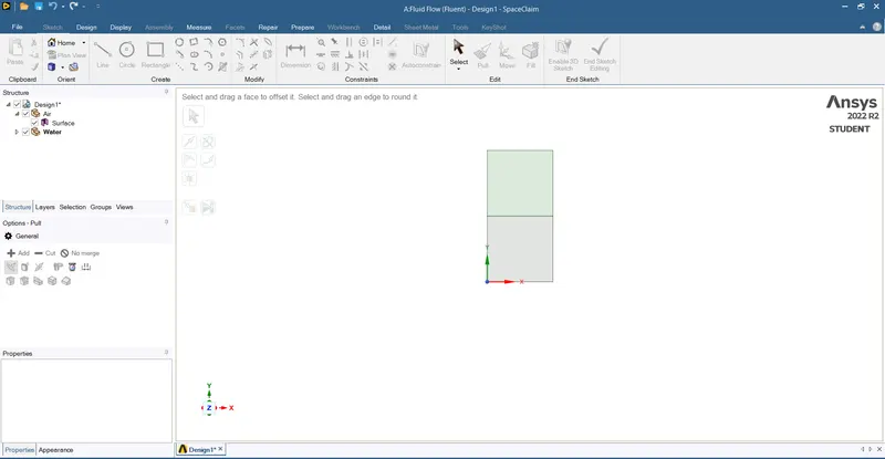
• Choose Fluent from the workbench setup, edit SpaceClaim to create geometry.
• Choose the XY plane to sketch 2Dgeometry, create a square of 20mm, and select pull tool to make it a surface of that.
• Move the geometry to a new component and rename it as Air.
• Now create new geometry under the main design as water and create a square of 20mm right on top of the air square which creates an interface between the 2 boxes.
• Select the entire geometry for share prep under the workbench and select share so that the interface can face information and conformal meshing can be achieved between the 2 phases.

2. Mesh

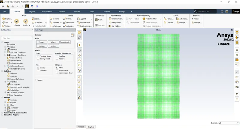
• OPEN MESH --> Generate the mesh --> baseline mesh element size 0.0005m(0.5mm).

3. et Up

• DOUBLE CLICK SETUP -- > FLUENT LAUNCHER -->DOUBLE PRECISION.
• Ansys Fluent is opened.
• In Graphics window --> GEOMETRY AND CONSOLE window is displayed.
• SETTING UP DOMAIN -->MESH --> select CHECK. Then in CONSOLE WINDOW --> it shows 'CHECKING MESH…. DONE'
• To Change the Units, SETTING UP DOMAIN --> click Units
• SETTING UP PHYSICS --> SOLVER --> select Time = Transient, Type = PRESSURE BASED & Velocity Formation = ABSOLUTE.
• VISCOUS MODEL --> Laminar--> OK.
• Multiphase--> Model=Volume of Fluid, select Implict Formulation, -->Number of Eulerian Process is 2.
• Phases --> primary phase=Air(phase-1) and secondary phase=Water(phase-2).
• Material selection. Materials -->Air and Water.
• Setting up Domain ---> go to Display --> check for all the zones.
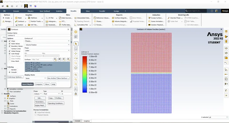
• Solving -->Method=standard --> Patch--> Phase=Water, Variable=Volume Fraction --> select water_surface=1 --> click Patch. Similarly for air_surface=0 --> click Patch.
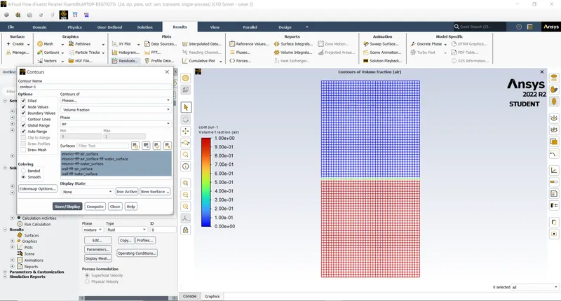
• Postprocessing --> create contours --> contour of= Phases, Phase=water, select all the surfaces --> Save/Display. Now contour is generated showing water at top and air at bottom.
• Solving --> select Method=standard > go to Patch --> Phase=Water, Variable=Volume Fraction --> select water_surface=1 > click Patch. Similarly select air_surface=0 > click Patch.

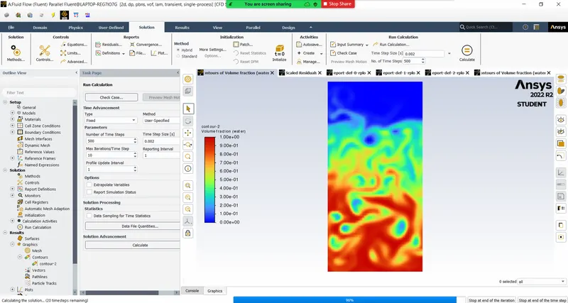
• Run-->Calculation > Type=Fixed Time STep, Time step Size=0.002, Number of iterations=500 --> click Calculate.

4. Solution

• SOLVING --> CONTROLS, REPORTS, INITIALIZATION, RUN CALCULATION.
• REPORTS-- > DEFINITIONS --> NEW --> SURFACE REPORT -->AREA WEIGHTED AVERAGE. Similarly, select STANDARD DEVIATION. For both the cases, a 'SURFACE REPORT DEFINITION WINDOW'pops up > select the FIELD VARIABLE = Temperature
• CREATE --> select REPORT FILE and REPORT PLOT.
• INITIALIZATION --> select METHOD = HYBRID --> click t=0 INITIALIZE
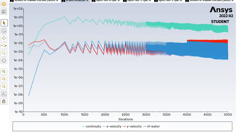
• RUN CALCULATION --> NO. OF ITERATIONS =500 and press CALCULATE.

5.Results and Discussion:

https://youtu.be/_-FoXaH3U0w