Project 2 - Rankine cycle Simulator
Aim:Write program in matlab for rankin cycle
Objective:
- Net work output
- Back work ratio
Theory:
The Rankine cycle is an idealized thermodynamics cycle describing the process by which certain heat engines such as steam turbines or reciprocating steam engines, allow mechanical work to be extracted from a fluid as it moves between a heat source and heat sink. The Rankine cycle is named after William John Macquorn Rankine, a Scottish polymath professor at Glasgow University. Heat energy is supplied to the system via a boiler where the working fluid (typically water) is converted to a high pressure gaseous state (steam) in order to turn a turbine. After passing over the turbine the fluid is allowed to condense back into a liquid state as waste heat energy is rejected before being returned to boiler, completing the cycle. Friction losses throughout the system are often neglected for the purpose of simplifying calculations as such losses are usually much less significant than thermodynamic losses, especially in larger systems.
Basic Cycle
The pressure-enthalpy (p-h) and temperature-entropy (T-s) diagrams of this cycle are given in fig 2. The Rankine cycle operates in the following steps:
-
1-2-3 Isobaric Heat Transfer. High pressure liquid enters the boiler from the feed pump (1) and is heated to the saturation temperature (2). Further addition of energy causes evaporation of the liquid until it is fully converted to saturated steam (3).
-
3-4 Isentropic Expansion. The vapor is expanded in the turbine, thus producing work which may be converted to electricity. In practice, the expansion is limited by the temperature of the cooling medium and by the erosion of the turbine blades by liquid entrainment in the vapor stream as the process moves further into the two-phase region. Exit vapor qualities should be greater than 90%.
-
4-5 Isobaric Heat Rejection. The vapor-liquid mixture leaving the turbine (4) is condensed at low pressure, usually in a surface condenser using cooling water. In well designed and maintained condensers, the pressure of the vapor is well below atmospheric pressure, approaching the saturation pressure of the operating fluid at the cooling water temperature.
-
5-1 Isentropic Compression. The pressure of the condensate is raised in the feed pump. Because of the low specific volume of liquids, the pump work is relatively small and often neglected in thermodynamic calculations.
Matlab Code:
clear all
close all
clc

%Input
disp('RANKINE CYCLE');
disp('1-2 is Isentropic Expansion in the turbine');
disp('2-3 is constant pressure heat removal in the condenser');
disp('3-4 is Isentropic compression in the pump');
disp('4-1 is Constant pressure heat addition in the boiler');

% Obtaining the input data
p1 = input('nValue of pressure at turbine inlet,p1(in bar) = ');
T1 = input('nValue of temperature at turbine inlet, T1(in degree.C) = ');
p2 = input('nValue pf temperature at condenser inlet, p2(in bar) = ');

% Extracting data_defining variables
% State 1
h1 = XSteam('h_pT',p1,T1);   %extracting enthalpy at state pt 1
s1 = XSteam('s_pT',p1,T1);    % same as above

%state 2
s2 = s1;      %Isentropic expansion
sf2 = XSteam('sL_p',p2);  %saturated liquid entropy
sg2 = XSteam('sV_p',p2);   %saturated vapour entropy
x2 = (s2-sf2)/(sg2-sf2);
hf2 = XSteam('hL_p',p2);
hg2 = XSteam('hV_p',p2);
h2 = hf2 + (x2*(hg2-hf2));

% state 3
p3 = p2;            % constant pressure heat rejection in condenser
s3 = XSteam('sL_p',p3);
h3 = XSteam('hL_p',p3);

%state 4
s4 = s3;
p4 = p1;

%Work done by turbine
Wt = h1-h2;

%work done to run pump
v3 = XSteam('vL_p',p3);
Wp = v3*(p4-p3)*100;
h4 = h3 + Wp;

%net work
Wnet = Wt - Wp;

%heat into of the system
Qin = h1-h3;

%thermal efficiency
eff = (Wnet/Qin)*100;

%specific steam consumption
%ssc = mass flow rate/power
SSC = (3600/Wnet);

%calculating temperature at the state point
T3 = XSteam('Tsat_p',p3);
T2 = T3;
Cp4 = XSteam('Cp_ps',p4,s4);
Cv4 = XSteam('Cv_ps',p4,s4);
k = Cp4/Cv4;
T4 = T3/((p3/p4)^((k-1)/k));

%calculating temperature,entropy and enthalpy at vapour
T6 = XSteam('Tsat_p',p1);
s5 = XSteam('sL_p',p1);
s6 = XSteam('sV_p',p1);
h5 = XSteam('hL_p',p1);
h6 = XSteam('hV_p',p1);
T5 = T6;

%plotting the saturation curve
T = linspace(1,375,1000);
for i = 1:length(T)

sf(i) = XSteam('sL_T',T(i));
sg(i) = XSteam('sV_T',T(i));
hf(i) = XSteam('hL_T',T(i));
hg(i) = XSteam('hv_T',T(i));
end

%plotting T-s diagram
figure(1)
hold on
plot(sf,T,'r','linewidth',1)
plot(sg,T,'r','linewidth',1)
plot([s1 s2],[T1 T2],'k','linewidth',2)
plot([s2 s3],[T2 T3],'k','linewidth',2)
plot([s3 s4],[T3 T4],'k','linewidth',2)
plot([s4 s5],[T4 T5],'k','linewidth',2)
plot([s5 s6],[T5 T6],'k','linewidth',2)
sc1 = linspace(s6,s1,1000);
for l = 1:length(sc1)
  Tc1(l) = XSteam('T_ps',p1,sc1(l));
end

plot(sc1,Tc1,'k','linewidth',2)
text(s1+0.1,T1,'1')
text(s2+0.1,T1,'2')
text(s3, T3-20,'3')
text(s4, T4+20,'4')
title('Temp vs Entropy plot')
xlabel('Entropy,S(Kj/kgk')
ylabel('Temperature (degree C)')
legend('Saturation curve')

%plotting h-s diagram
figure(2)
hold on
plot(sf,hf,'r','linewidth',1)
plot(sg,hg,'r','linewidth',1)
plot([s1 s2],[h1 h2], 'k', 'linewidth', 2)
plot([s2 s3],[h2 h3], 'k', 'linewidth', 2)
plot([s3 s4],[h3 h4], 'k', 'linewidth', 2)
hc = linspace(h4, h5, 100);
for k = 1:length(hc)
sch(k) = XSteam('s_ph', p1, hc(k));
end
plot(sch,hc, 'k', 'linewidth', 2)
plot([s5 s6], [h5 h6], 'k', 'linewidth',2)
for m=1:length(sc1)
    hc1(m)= XSteam('h_ps',p1, sc1(m));
end
plot(sc1,hc1, 'k', 'linewidth', 2)
text(s1+0.1, h1, '1')
text(s2+0.1, h2, '2')
text(s3+0.1, h3, '3')
text(s4+0.1, h4, '4')
title('Enthalpy vs Entropy plot')
xlabel('Entropy , S(KJ/kgk)')
ylabel('Enthalpy , H(KJ/kg)')
legend('Saturation curve', 'location','northwest')

% Display results
disp('RESULTS');
fprintf('At State Point 1:n');
fprintf('p1: %8.3f barn',p1);
fprintf('T1: %8.3f Cn',T1);
fprintf('h1: %8.3f kJ/kgn',h1);
fprintf('s1: %8.3f kJ/kgKnn',s1);
fprintf('At State Point 2:n');
fprintf('p2: %8.3f barn',p2);
fprintf('T2: %8.3f Cn',T2);
fprintf('h2: %8.3f kJ/kgn',h2);
fprintf('s2: %8.3f kJ/kgKn',s2);
fprintf('x2: %8.3fnn',x2);
fprintf('At State point 3:n');
fprintf('p3: %8.3f barn',p3);
fprintf('T3: %8.3f kn',T3);
fprintf('h3: %8.3f kJ/kgn',h3);
fprintf('s3: %8.3f kJ/kgKnn',s3);
fprintf('At State Point 4:n');
fprintf('p4: %8.3f barn',p4);
fprintf('T4: %8.3f kn',T4);
fprintf('h4: %8.3f kJ/kgn',h4);
fprintf('s4: %8.3f kJ/kgKnn',s4);
fprintf('Turbine Work: %8.3f kJ/kgn',Wt);
fprintf('Pump Work: %8.3f kJ/kgn',Wp);
fprintf('Wnet: %8.3f kJ/kgn',Wnet);
fprintf('Efficiency: %8.3f Percent n',eff);
fprintf('S.S.C: %8.3f kJ/kWh',SSC);
Output:
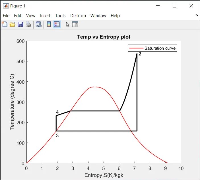
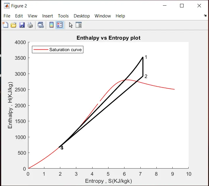
RANKINE CYCLE
1-2 is Isentropic Expansion in the turbine
2-3 is constant pressure heat removal in the condenser
3-4 is Isentropic compression in the pump
4-1 is Constant pressure heat addition in the boiler
nValue of pressure at turbine inlet,p1(in bar) = 44
nValue of temperature at turbine inlet, T1(in degree.C) = 538
nValue pf temperature at condenser inlet, p2(in bar) = 5.83
RESULTS
At State Point 1:
np1:   44.000 barn
T1:  538.000 Cn
h1: 3528.829 kJ/kgn
s1:    7.154 kJ/kgKnnAt

State Point 2:n
p2:    5.830 barn
T2:  157.712 Cn
h2: 2920.821 kJ/kgn
s2:    7.154 kJ/kgKn
x2:    1.079nnAt

State point 3:
np3:    5.830 barn
T3:  157.712 kn
h3:  665.638 kJ/kgn
s3:    1.920 kJ/kgKnnAt


State Point 4:np4:   44.000 barnT4:  232.874 knh4:  669.834 kJ/kgns4:    1.920 kJ/kgKnn
Turbine Work:  608.008 kJ/kgn
Pump Work:    4.196 kJ/kgn
Wnet:  603.812 kJ/kgn
Efficiency:   21.089 Percent n
S.S.C:    5.962 kJ/kWh>>
>>
Refrences: