Week 3 - Solving second order ODEs

Aim: Write a matlab program to simulate the transist behaviour of simple pendulum.

Objective: 1) Create animation of its motion.

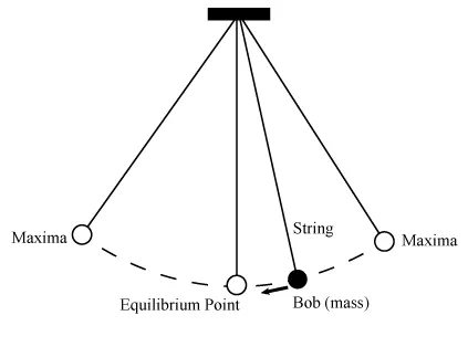
Theory: The simple pendulum is a mechanical system that sways or moves in an oscillatory motion. This motion occurs in a vertical plane and is mainly driven by the gravitational force. Interestingly, the bob that is suspended at the end of a thread very light somewhat we can say it is even massless. The period of a simple pendulum can be made extended by increasing the length string while taking the measurements from the point of suspension to the middle of the bob. However, it should be noted that if the mass of the bob is changed it will the period remains unchanged. Period is influenced mainly by the position of the pendulum in relation to Earth as the strength of gravitational field is not uniform everywhere.

Terms are used in pendulum:

The oscillatory motion of a simple pendulum: Oscillatory motion is defined as the to and fro motion of the pendulum in a periodic fashion and the centre point of oscillation known as equilibrium position.
The time period of a simple pendulum: It is defined as the time taken by the pendulum to finish one full oscillation and is denoted by “T”.
The amplitude of simple pendulum: It is defined as the distance travelled by the pendulum from the equilibrium position to one side.
Length of a simple pendulum: It is defined as the distance between the point of suspension to the centre of the bob and is denoted by “l".

Mathematical Expression:

n the above equation,

g = gravity in m/s2,

L = length of the pendulum in m,

m = mass of the ball in kg,

b=damping coefficient.

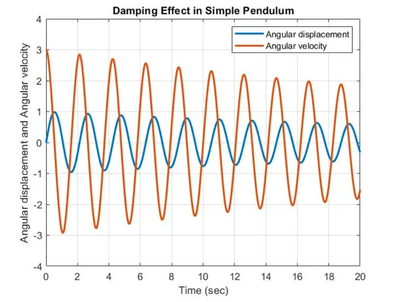
Simulate the motion between 0-20 sec, for angular displacement=0,angular velocity=3 rad/sec at time t=0.

Matlab Code :

clear all
close all
clc

%inputs
b = 0.05;
g = 9.81;
l = 1;
m = 1;

% initial condition
theta_0 = [0;3];

%time point
t_span = linspace(0,20,600);

%solving ODE
[t,y] = ode45(@(t,theta) ode_func(t,theta,b,g,l,m),t_span,theta_0);

%Plotting Angular Displacement and Angular Velocity w.r.t
plot(t,y(:,1),'linewidth',2);
hold on
plot(t,y(:,2),'linewidth',2);
axis([0 20 -4 4]);
xlabel('Time (sec)');
ylabel('Angular displacement and Angular velocity');
grid on
title('Damping effect in simple pendulum');
legend('Angular displacement','Angular velocity');
pause(15);

ct = 1;
for i = 1:length(t_span);
    
    x0 = 0
    y0 = 0
    
    x1 = l*sin(y(i,1));
    y1 = -l*cos(y(i,1));
    
    %simulation of motion of pendulum
    plot([x0 x1],[y0 y1],[-0.5 0.5],[0 0],'linewidth',3)
    hold on
    plot(x1,y1,'marker','o','markerSize',25,'markerFacecolor','r')
    axis([-1.5 1.5 -1.5 0.5])
    grid on
    title('Motion of Simple Pendulum with Damping')
    pause(0.01)
    M(ct) = getframe(gcf);
    ct = ct +1;
    hold off
    
end

%Animation of motion of simple pendulum
movie(M)
videofile = VideoWriter('Simple_Pendulum.avi','Uncompressed AVI')
open(videofile)
writeVideo(videofile,M)
close(videofile)

• Program start with clear all , close all ,clc command.
• Then we give input value to program b,g,l,m,theta and time.
• write ODE equation to solve expression.
• use plot command to create plot .
• for loop to create animation.
• Video command

Sub Code for Function

function [dtheta_dt] = ode_func(t,theta,b,g,l,m)
theta1 = theta(1)
theta2 = theta(2)
dtheta1_dt = theta2
dtheta2_dt = -(b/m)*theta2 - (g/1)*sin(theta1);
dtheta_dt = [dtheta1_dt;dtheta2_dt];
end

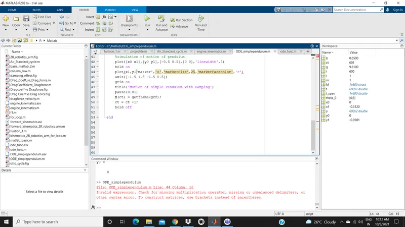
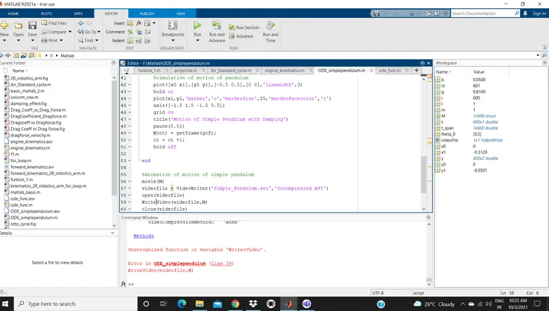
Errors:

Output:

Animation Link: https://youtu.be/30OfPG5CVbA

Refrence: Google Search Engine