Week 5 - Rayleigh Taylor Instability

Aim:

1. What are some practical CFD models that have been based on the mathematical analysis of Rayleigh Taylor waves? In your own words, explain how these mathematical models have been adapted for CFD calculations.
2. Perform the Rayleigh Taylor instability simulation for 2 different mesh sizes with the base mesh being 0.5 mm. Compare the results by showing the animations( Attach them from your google drive). Observe the differences in the animation and explain the effect of mesh size on simulation. Also, explain why a steady-state approach might not be suitable for these types of simulation.[ Choose Air and Water for this simulation]
3. Run one more simulation with water and user-defined material(density = 400 kg/m3, viscosity = 0.001 kg/m-s) for refined mesh.
4. Define the Atwood Number. Find out the Atwood number for both the cases and explain how the variation in Atwood number in the above two cases affects the behavior of the instability.

Explanation and solutions

Rayleigh Tayler instability

Rayleigh-Taylor instability (RTI) is the interpenetration of materials that occurs whenever a light fluid pushes on a heavy fluid (Rayleigh 1883, Taylor 1950). It is a dynamic process whereby the two fluids seek to reduce their combined potential energy. The ensuing turbulence and mixing has far-reaching consequences in many natural and man-made flows, ranging from supernovae to inertial confinement fusion (ICF) capsules.

Practical CFD models that have been based on mathematical analysis of RT waves.

1. Kelvin-Helmholtz instability
2. Richtmyer-Meshkov instability
3. Plateau-Rayleigh instability

1. Kelvin-Helmholtz instability

The Kelvin–Helmholtz instability (after Lord Kelvin and Hermann von Helmholtz) can occur when there is velocity shear in a single continuous fluid, or where there is a velocity difference across the interface between two fluids. An example is wind blowing over water: The instability manifests in waves on the water surface. More generally, clouds, the ocean, Saturn's bands, Jupiter's Red Spot, and the sun's corona show this instability.

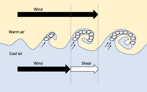
Formation of Kelvin Helmholtz waves and associated "billow" clouds When the rising cooler air is moist, under the correct conditions, cloud forms in the crest of each wave. To the viewer on the ground, these appear as parallel bands of cloud. The waves break on top into cloud rolls. The axes of the cloud rolls are perpendicular to the wind shear.

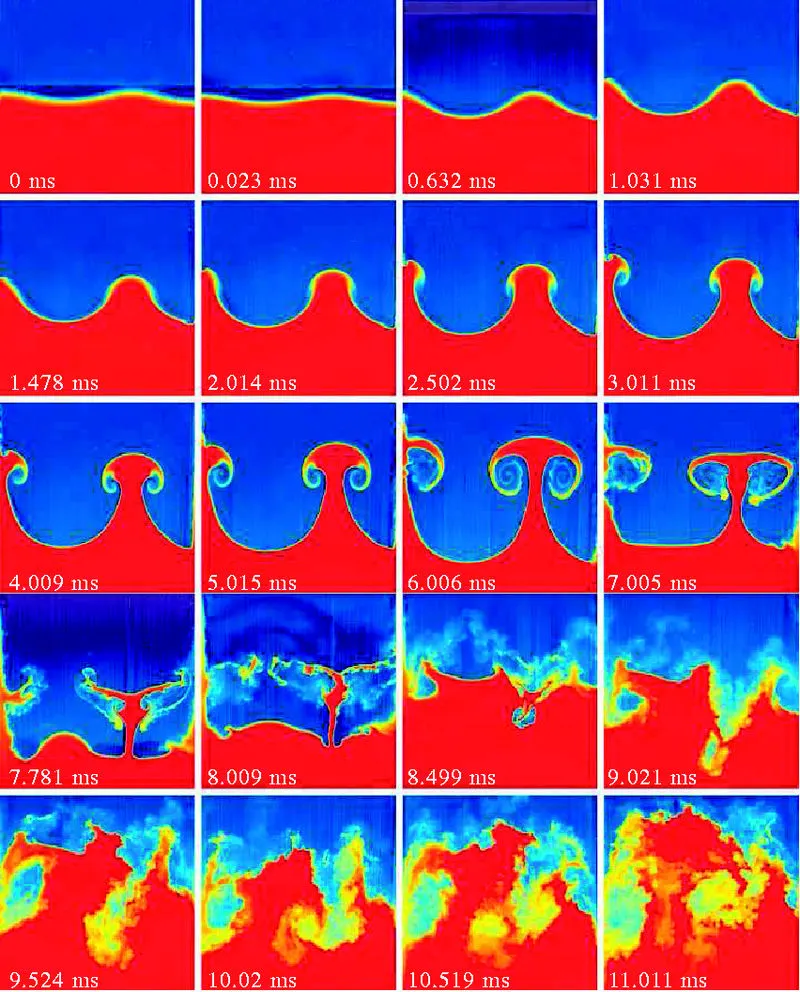
1. Richtmyer-Meshkov instability- This occurs when two fluids of different density are impulsively accelerated. Normally this is by the passage of a shock wave. The development of the instability begins with small amplitude perturbations which initially grow linearly with time. This is followed by a nonlinear regime with bubbles appearing in the case of a light fluid penetrating a heavy fluid, and with spikes appearing in the case of a heavy fluid penetrating a light fluid. A chaotic regime eventually is reached and the two fluids mix. This instability can be considered the impulsive-acceleration limit of the Rayleigh Taylor instability.

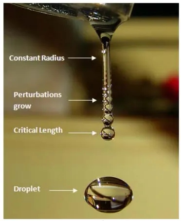
1. Plateau-Rayleigh instability

The Plateau–Rayleigh instability of a liquid column underlies a variety of fascinating phenomena that can be observed in everyday life. In contrast to the case of a free liquid cylinder, describing the evolution of a liquid layer on a solid fibre requires consideration of the solid–liquid interface. Here we revisit the Plateau–Rayleigh instability of a liquid coating a fibre by varying the hydrodynamic boundary condition at the fibre–liquid interface, from no slip to slip. Although the wavelength is not sensitive to the solid–liquid interface, we find that the growth rate of the undulations strongly depends on the hydrodynamic boundary condition. The experiments are in excellent agreement with a new thin-film theory incorporating slip, thus providing an original, quantitative and robust tool to measure slip lengths.

Procedure

1. Geometry:-
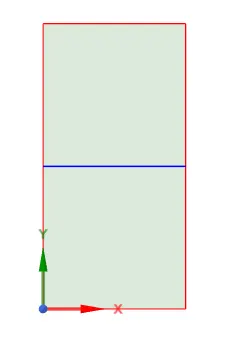
• Select X-Y plan and create the geometry.
• Open space claim and create 2 square one representing water which is on top of another which is representing air.
• And pull to create the surface.
• Put on the share topology.
• 

2. Meshing:-

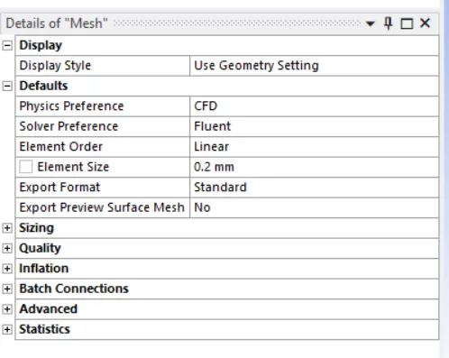
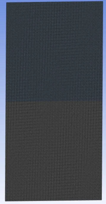
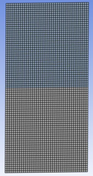
   • Create base line mesh of 0.5 mm. and then decrease the size to 0.2 to 0.3 mm for better results.

   • 

   • 0.2mm Mesh

   • 

   • 0.5 mm mesh.

   • 

3. Fluent Setup

   • Solver:- Pressure based solver with transient state.
   • Put on the gravity setting and assign the value of gravity as 9.81 m/s.
   • Physics:- use laminar model for solving.
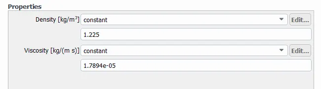
   • Material used:- water and Air (select Water from fluent data base)

     • Material properties-Air

     • 

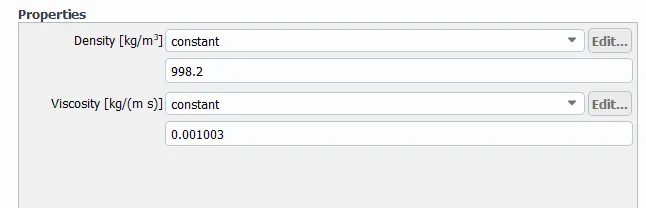
     • Material properties-Water

       • Material properties-Water
     • 

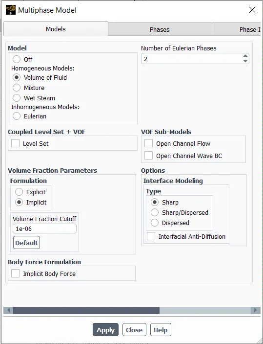
   • Set Multiphase settings as per the below image.

     • • Model - Volume of fluid
       • Formulation - implicit
       • Number of eulerian phases:-

       This is available only with the density-based solver. Number of Eulerian Phases allows you to specify the number of phases for the multiphase calculation. You can specify up to 20 phases.

     • 

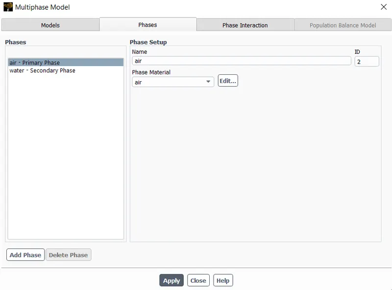
     • Phases.

     • 

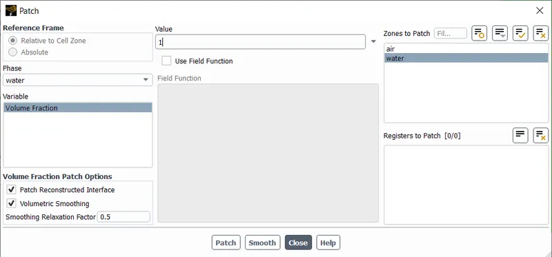
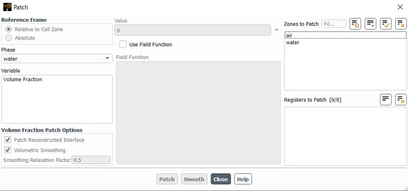
     • Initialize and patch the zones

     • 
     • 

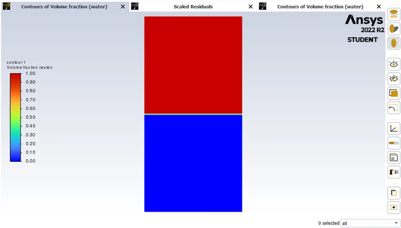
     • Set Contour

     • 

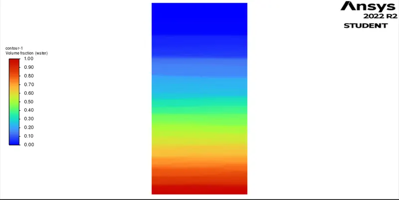
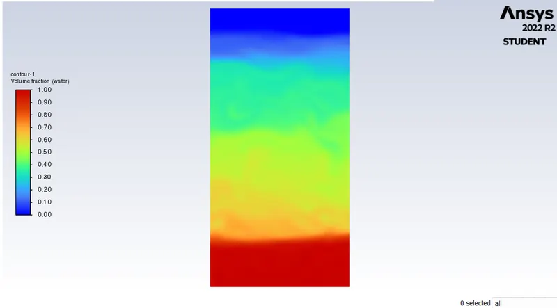
     • Contour After the finish of simulation for 0.5 mm mesh ..

     • 

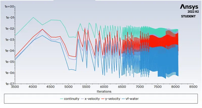
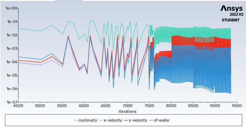
     • Residual chart for 0.5mm mesh

     • 

     • Contour of user defined material

       • 

     • Residual

       • 

• Video Links

1. Animation for water and air with 0.5 mm mesh size.

https://drive.google.com/file/d/1XuxXjyERcNgUNS7bUNBROvDjfoo_F4Gb/view?usp=sharing

2. Animation for water and air with 0.3 mm mesh size

https://drive.google.com/file/d/1C6iVij0kx-3rTGZ_2fUYckvVOHovF--s/view?usp=sharing

3. Animation for water and user defined material.

https://drive.google.com/file/d/1QAJjFyk28L4CCOo7kuVOV7J4GV0_f0QT/view?usp=sharing

Atwood number

• The Atwood number (A) is a dimensionless number in Fluid dynamics used in the study of hydrodynamic instability in density stratified flows. It is a dimensionless density ratio defined as
• 
• 
• 

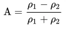
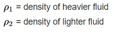
• Atwood number is an important parameter in the study of rayleigh-tayor instability and richmyer-mechkow instability. In RTI, the penetration distance of heavy fluid bubbles into the light fluid is a function of acceleration time scale, where g is the gravitational acceleration & t is the time.

Conclusion

• As mesh become finer, the mixing becomes much clear & visible.
• The computation time also increases with increases in finer of mesh.