Week 5 - Rayleigh Taylor Instability
CHALLENGE REPORT :
AIM :
To perform the Rayleigh Taylor instability simulation and compare the results.
OBJECTIVE :
* To explain about some of the practical CFD models that have been based on the mathematical analysis of Rayleigh Taylor wave.
* To perform the Rayleigh Taylor instability simulation for 2 different mesh sizes with the base mesh being 0.5 mm.
* Comparing the results by using the animations and observe the differences in the animation and explain the effect of mesh size on the simulation.
* Explaing the reson why the steady state approach is not used for these type of simulation.
* The information about the Atwood number for both the cases and the variation in Atwood number in the above two cases affects the behavior of the instability is explained.
THEOREY :
RAYLEIGH TAYLOR INSTABILITY :
The Rayleigh–Taylor instability, or RT instability, is the instability of an interface between two fluids of different densities which occurs when the lighter fluid is pushing the heavier fluid. Examples include the behavior of water suspended above oil in the gravity of the earth, mushroom clouds like those from a volcanic eruption and atmospheric nuclear explosion, supernova explosions in which expanding core gas is accelerated into denser shell gas, instabilities in plasma fusion reactors, and inertial confinement fusion.
EXAMPLE :
Water suspended top oil is an everyday example of Rayleigh–Taylor instability, and it may be modeled by two completely plane-parallel layers of immiscible fluid, the denser on top of the less dense one and both subject to the Earth's gravity. The equilibrium here is unstable to any perturbations or disturbances of the interface: if a parcel of heavier fluid is displaced downward with an equal volume of lighter fluid displaced upwards, the potential energy of the configuration is lower than the initial state. Thus the disturbance will grow and lead to a further release of potential energy, as the more dense material moves down under the (effective) gravitational field, and the less dense material is further displaced upwards. This was the set-up as studied by Lord Rayleigh.
Types of Instability and some practical CFD models that have been based on the mathematical analysis of Rayleigh Taylor waves:
Ritchmyer-Meshkov instability:
The Richtmyer-Meshkov instability arises when a shock wave interacts with an interface separating two different fluids. It combines compressible phenomena, such as shock interaction and refraction, with hydrodynamic instability, including nonlinear growth and subsequent transition to turbulence, across a wide range of Mach numbers.
Plateau–Rayleigh instability:
The Plateau–Rayleigh instability, often just called the Rayleigh instability, explains why and how a falling stream of fluid breaks up into smaller packets with the same volume but less surface area. This fluid instability is exploited in the design of a particular type of inkjet technology whereby a jet of liquid is perturbed into a steady stream of droplets.
Kelvin–Helmholtz instability:
Kelvin–Helmholtz instability can occur when there is velocity shear in a single continuous fluid, or where there is a velocity difference across the interface between two fluids. An example is a wind blowing over water: The instability manifests in waves on the water's surface. More generally, clouds, the ocean, Saturn's bands, and the sun's corona show this instability.
MULTIPHASE FLOW :
It is defined as the fluid flow where the simultaneous flow of materials with two or more thermodynamic phases exist together.
Example of Multi-phase Flow: Water bubble column, boiling and condensation and cavitation pump and turbine etc.
TYPES OF PHASES IN MULTIPHASES :
* Separated phases,
* Mixed phases,
* Dispersed phases.
VOLUME OF FLUID (VOF) :
The volume of fluid (VOF) method is a free surface modelling technique, i.e. a numerical techinques for tracking and locating the free surface (or fluid fluid interfaces). It belongs to the class of Eulerian methods which are characterized by a mesh that is either stationary or is moving in a certain prescribed manner to accommodate the evolving shape of the interface. As such, VOF is an advection scheme—a numerical recipe that allows the programmer to track the shape and position of the interface, but it is not a standalone flow solving algorithm.
Atwood Number :
Dealing with mixtures of fluid one uses the Atwood number to characterize the density difference between two fluids.
Assume that rho_2 is the density of the heavier fluid.
The definition is: At = (rho_2 - rho_1) / (rho_2 + rho_1).
- For big density differences Atwood number tends to 1.
- For small differences Atwood number tends to zero.
PROCEDURE :
GEOMENTRY SETUP :
* Geomentry is created by opening the space claim .
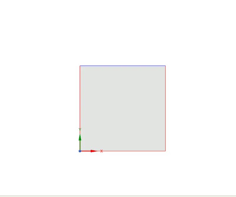
* Create a square with 20x20 by square option in the sketch mode and using the pull or applying the return to 3D, convert it as model. Make it as seperate component and name it as air.
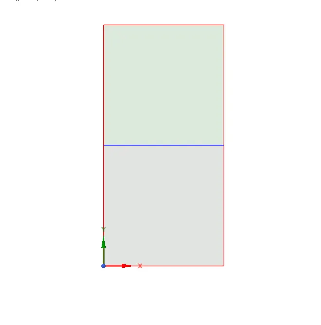
* Create other square with same dimension above thw air surface and apply the return to 3D. Make it as seperate component and name it as water.
MESH :
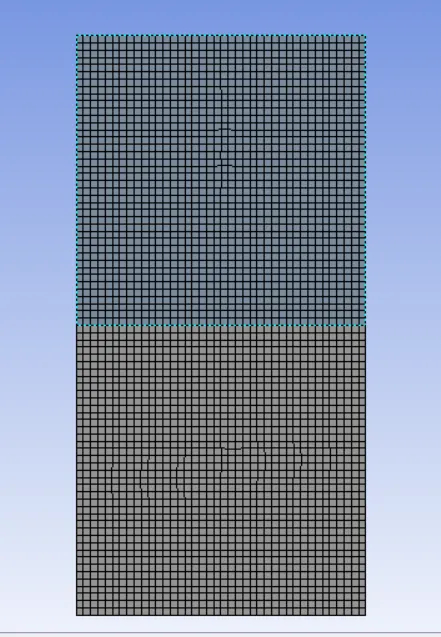
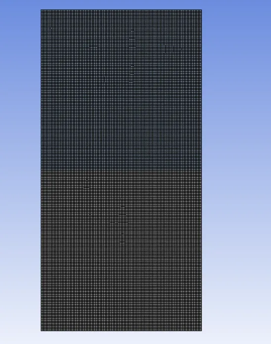
* Created geomentry is open in the mesh and give generate mesh.
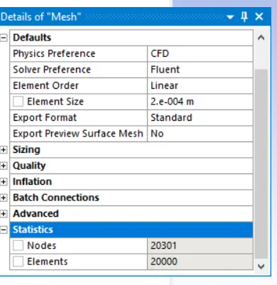
* Here mesh independent study is done by cases of different element size.
Two different element size :
Case 1:
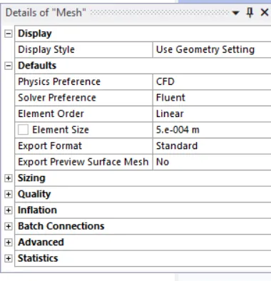
element size =0.5mm
Case 2:
element size =0.2mm
| CASES | ELEMENT SIZE | NUMBER OF ELEMENTS |
| 1 | 0.5mm | 3200 |
| 2 | 0.2mm | 20000 |
SETUP SOLUTION :
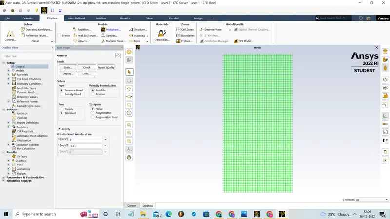
* After the mesh open the set up modul and here we have to set the condition like physics, boundery conditions, type of analysics, Solution setups and the requried outups.
* Here enable the transient solver because we need simulation results for each and every seconds so we nned to consider the changes in every time (sec). Pressure based is used because the velocity of air low ( less than 0.3 of mach number ) and enable gravity with Y axis as -9.81 .
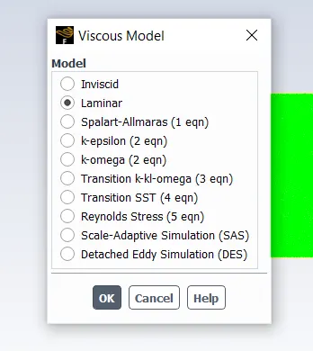
* Use laminar model by opening the Viscous option in the physics.
* Choose the material from the material selection. Seect the material using the fluent database which as default materials. Two cases of materials is to be selected as per problem statement.
Two type of Cases.
Case1 :
Materials used : Air and Water with the default properties.
Case2 :
Materials used : Water with the default properties and User defined material with given properties.
| MATERIALS | DENSITY (Kg/m^3) | VISCOSITY (Kg/ms) |
| Air | 1.225 | 1.7894e-05 |
| Water | 998.2 | 0.001003 |
| User defined material | 400 | 0.001 |
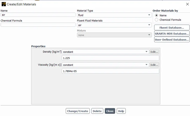
* Select the multiphase and change to volume of fluid. In that select the implicit method, so that we don't need to depends on the courant number, we can use suitable time step size. In the phase choose the phase and apply it.
* Just initialize it by selecting the initialize option in solution tab.
* Patch as to done as by selection water and volume frature. set the water as 1 and air as 0 as apply patch.
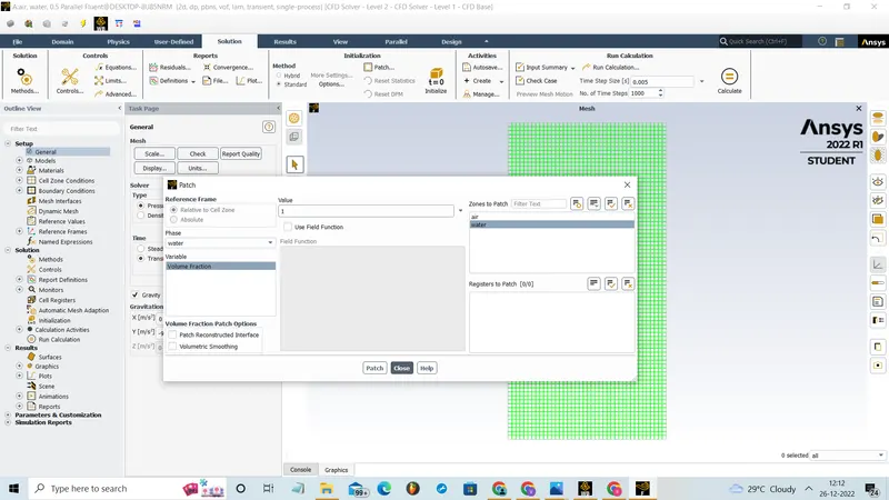
* Select the time step number and set as 0.005s and no of time step is 1000 and run the simulation.
* Create the solution animation from the create option with 1 time step ans apply active option.
RESULTS :
MESH INDIPENDENT STUDY :
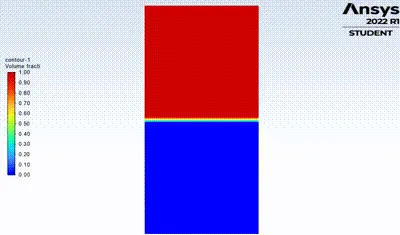
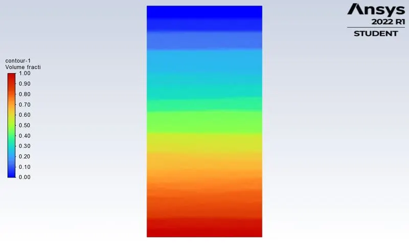
From the mesh indipendent study we can see that volume frature and instability betweeen the fluids can be anlysed very accurately and clearly from the fine mesh size. The bubble formation and the water bulles formation during these multiphase process can be much more clearly analysed using these fine mesh size of 0.2mm when compare to base mesh of 0.5mm. so we can use the 0.2mm mesh size for further simulation process.
CASE 1 :
MESH SIZE =0.5MM
MATERIALS = Air and Weter
RESIDUAL PLOT :
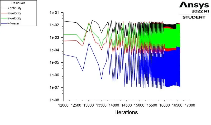
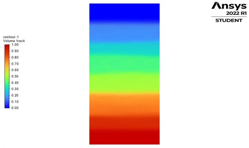
CONTOUR :
CASE 2 :
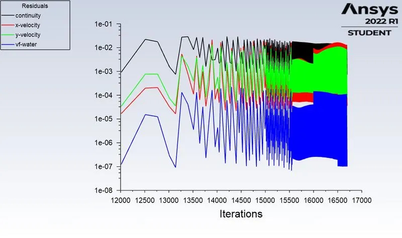
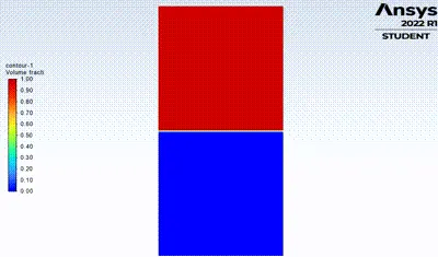
MESH SIZE =0.2MM
MATERIALS = Air and Weter
RESIDUAL PLOT :
CONTOUR :
CASE 3 :
MESH SIZE =0.2MM
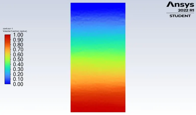
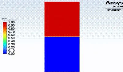
MATERIALS = User defin material and Weter
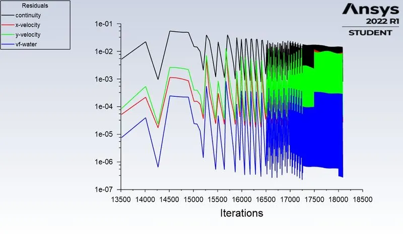
RESIDUAL PLOT :
CONTOUR :
Atwood Number:
It is a dimensionless number that is used to study hydrodynamic instabilities in density stratified flows.
It is denoted by letter A
A=(rho_1-rho_2)/(rho_1+rho_2)
where,
rho_1=Density of heavier fluid `
rho_2=Density of lighter fluid
The Atwood Number for Air-water RT instability
rho_1=998.2 (kg)/(m^3) (water density)
rho_2=1.225 (kg)/(m^3) (Air density)
A=(998.2 - 1.225) / (998.2+1.225)
we get A=0.9975
The Atwood Number for Water-UD material RT instability
rho_1=998.2 (kg)/(m^3) (Water density)
rho_2=400 (kg)/(m^3) (User defined material density)
A= (998.2 - 400) / (998.2+400)
we get A=0.4278
The Atwood number close to 1 then the lighter fluid below the heavier fluid which forms a larger bubbles which is less symmetrical and also it occurs very rapidly.
The Atwood number close to 0 then the lighter fluid below the heavier fluid which forms a bubbles which is relatively symmetrical and the pertubations are linear for larger time.
OBSERVATION :
* The finer mesh captures the instability better than the coarse mesh.but it takes more time for the heavier fluid to settle down.
* The computational time is also increased for fine mesh but the result obtained having better accuracy.
* The steady state simulation is performed if we are concerned more about the final state results or the equilibrium state,In RT instability CFD model we are more concerned to learn about the transition of the irregularities that start developing when we pour the high densiy fluid upon the low density fluid under the effect of gravity and we want to know how the interface collapses as a function of time. so In this case Transient state is more suitable over the steady state.
CONCLUSION :
* It is observed that the more we refine the mesh, the more the simulation results get smoother about the irregularities that take place at the interface of the two fluids. As higher-density fluid replaces lower-density fluid, the formation of air bubbles and vortex takes place, which travels towards the upward region with time.
* In the Rayleigh- Taylor Instability, due to a sudden collapse in the layer between the denser and lighter fluid spike generation takes place which is obviously time-dependent, hence using a steady state solver will not work as we are interested in the flow parameters with respect to time.
* For air- water Atwood number is 0.995 which is close to 1, so more bubbles is formed which is less symmetrical and also it occurs very rapidly.
* For water- Ud Atwood number is 0.4278 which is close to 0, so bubbles is formed which is relatively symmetrical and the pertubations are linear for larger time.