Week 5 - Rayleigh Taylor Instability
AIM: Define rayleigh taylor instability. In this project use laminar,Volume of fluid methd to understand the rayleigh taylor instability at the interface of the two fluids having diffrent densities at the Ansys fluent Tool.Also perform the mesh independent study to obtain the optimum results from the Ansys fluent.Define the Atwood number and variation of atwood number.
PROBLEM STATEMENT:
- What are some practical CFD models that have been based on the mathematical analysis of Rayleigh Taylor waves? In your own words, explain how these mathematical models have been adapted for CFD calculations.
- Perform the Rayleigh Taylor instability simulation for 2 different mesh sizes with the base mesh being 0.5 mm. Compare the results by showing the animations( Attach them from your google drive). Observe the differences in the animation and explain the effect of mesh size on simulation. Also, explain why a steady-state approach might not be suitable for these types of simulation.[ Choose Air and Water for this simulation]
- Run one more simulation with water and user-defined material(density = 400 kg/m3, viscosity = 0.001 kg/m-s) for refined mesh.
- Define the Atwood Number. Find out the Atwood number for both the cases and explain how the variation in Atwood number in the above two cases affects the behavior of the instability.
Introduction Theory:
A Rayleigh taylor instability occurs when the fluid of heavier density penetrates the fluid of lower density when the fluid accelerates in this case it is gravity.There are mainlt four stages. In the stage 1 start with the two fluid layers the upper 1 has highier density then the lower one, The rayleigh taylor instability occur given a small penetration because of diffrence in density there is diifrence in pressure at diifrent locations.
Another way to see the Rayleigh taylor instability with the eyes of vorticity. Vorticity is defined as the rotation of the velocity of the fluid layer.
The misalignment of the pressure and density gradient in the two fluid layers will cause a torque at the interface Which in turn create vorticity.This way of viewing the rayleigh taylor instability is generally used to find the numerical formulas.
All the numerical equations are used in the 2D but as we move to the second stage there are diffrent problems those are arrises at the 2D.To correctly define the formation of spikes and bubbles those are formed we have to move to the 3D spherical pictures.
During the third stage we will introduce to another stability that is kelvin helmholtz instability. This stability occur when two fluids have diffrent velocity component in the direction parallel to the interface.The effect of kelvin helmholtz instability that cause the spikes to form the characteristic curve arround the mushroom clouds.
In the fourth stage the spikes were breakup and the heavier fluid will dissolve in to lighter fluid.
>
As the RT instability develops, the initial perturbations progress from a linear growth phase into a non-linear growth phase, eventually developing "plumes" flowing upwards (in the gravitational buoyancy sense) and "spikes" falling downwards. In the linear phase, the fluid movement can be closely approximated by llinear equation and the amplitude of perturbations is growing exponentially with time. In the non-linear phase, perturbation amplitude is too large for a linear approximation, andnon linear equations are required to describe fluid motions. In general, the density disparity between the fluids determines the structure of the subsequent non-linear RT instability flows (assuming other variables such as surface tension and viscosity are negligible here). The difference in the fluid densities divided by their sum is defined as the Atwood no A. For A close to 0, RT instability flows take the form of symmetric "fingers" of fluid; for A close to 1, the much lighter fluid "below" the heavier fluid takes the form of larger bubble-like plumes.
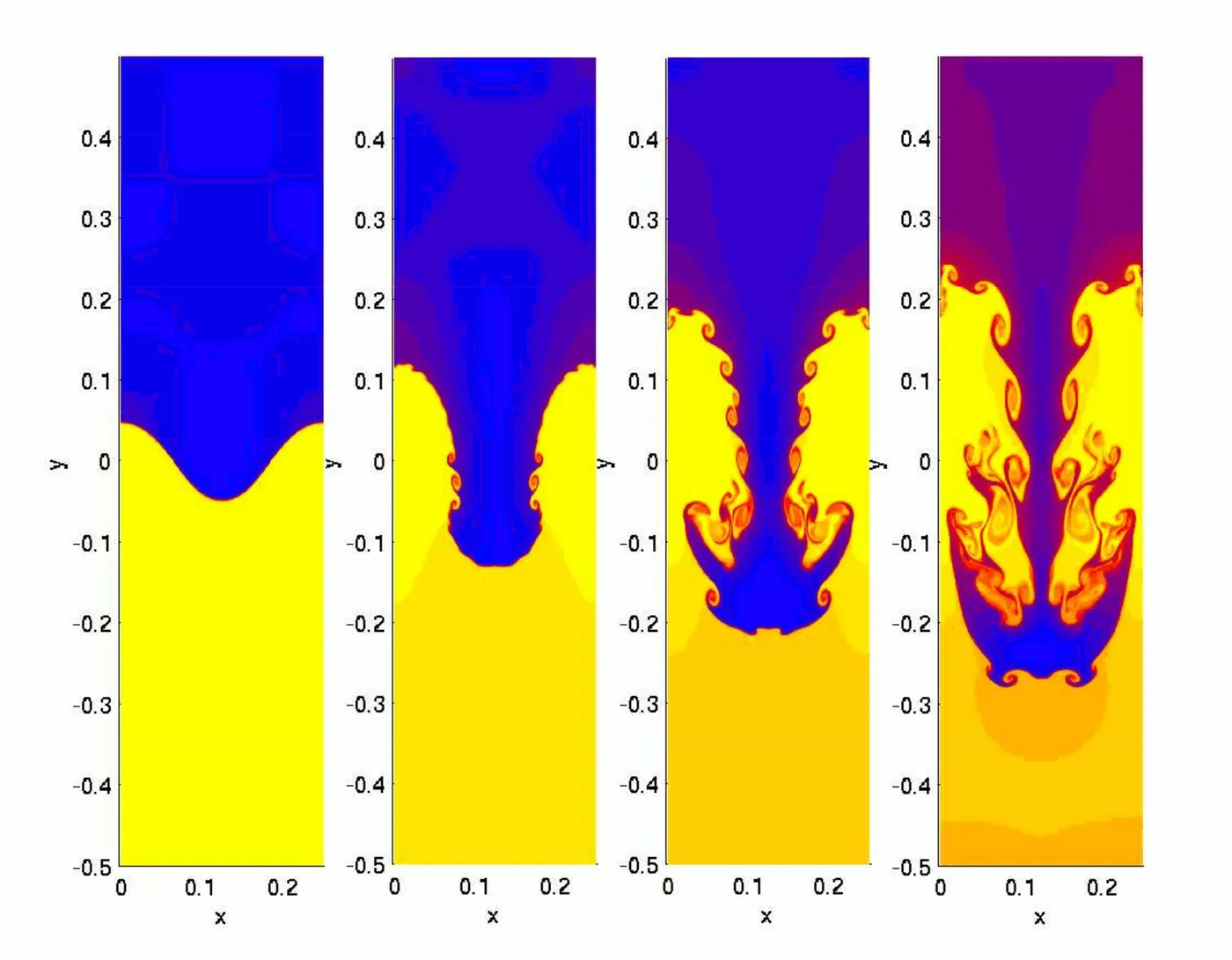
Some popular models of Rayleigh-Taylor instability are as follows:
- The Richtmyer–Meshkov instability (RMI) occurs when two fluids of different density are impulsively accelerated. Normally this is by the passage of a shock wave. The development of the instability begins with small amplitude perturbations which initially grow linearly with time. This is followed by a nonlinear regime with bubbles appearing in the case of a light fluid penetrating a heavy fluid, and with spikes appearing in the case of a heavy fluid penetrating a light fluid. A chaotic regime eventually is reached and the two fluids mix. This instability can be considered the impulsive-acceleration limit of the R-T instability.
- The Kelvin–Helmholtz instability typically occurs when there is velocity shear in a single continous fluid or additionally where there is a velocity difference across the interface between two fluids. A common example is seen with wind blowing over water, the instability constant is able to manifest itself through waves on a water surface. The Kelvin-Helmholtz instability is not only restricted to a water surface as clouds, but is evident through other natural phenomena as the ocean, Saturn's bands,Jupiters red spot, and the sun's corona.The Kelvin-Helmholtz instability phenomena is an all encompassing occurrence of fluid flow seen time and time again in nature. From the waves of the ocean to the clouds above in the sky, the Kelvin-Helmholtz instability is responsible for some of nature's most basic structures. Further analysis and modeling of the Kelvin-Helmholtz instability can result in an understanding of the worlds natural phenomena and more.
-
The Plateau–Rayleigh instability, often just called the Rayleigh instability, explains why and how a falling stream of fluid breaks up into smaller packets with the same volume but less surface area. It is related to theR-T instability and is part of a greater branch of fluid dynamics concerned with fluid breakup. This fluid instability is exploited in the design of a particular type of ink technology, whereby a jet of liquid is perturbed into a steady stream of droplets.The driving force of the Plateau–Rayleigh instability is that liquids, by virtue of their surface tensions, tend to minimize their surface area. A considerable amount of work has been done recently on the final pinching profile by attacking it with similar solutions.
Modelling and problem solving approach:
GEOMETRY CREATION:
> OPEN SPACECLAIM
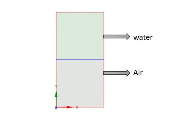
> Create a square of 20*20mm and use pull tool to convert it to in to 2D surface.
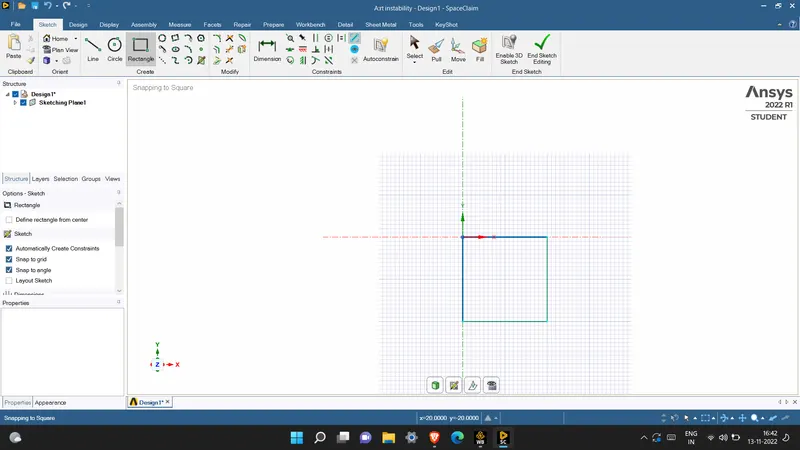
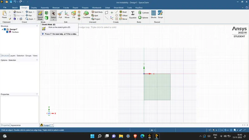
> go to surface right click on it it shows new component in the pop up window where give name as air.
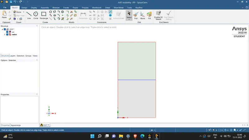
> go to design right click on it click on the new component and give name of the new componen as water
> click on water do to design click on sketch and create a square for the water.
> we want to create a formal mesh at the interface of two squares that we have created to create the conformal mesh at the interface we have to option.
1) use share tool present in the workbench. share topology will enable automatically.
2) enable share topology manually by design > sharetopology > enable
> To check whether the share topology enable automatically or not using first method go to design and check for share topology.
Meshing:
Case 1: meshing with element size of 0.5mm.
- Open the meshing console.
- Click on the mesh and select generate mesh option.
- Now a basic mesh pattern will be created as shown in image.
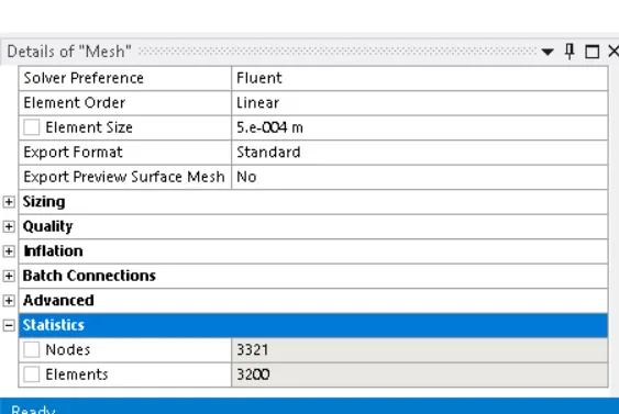
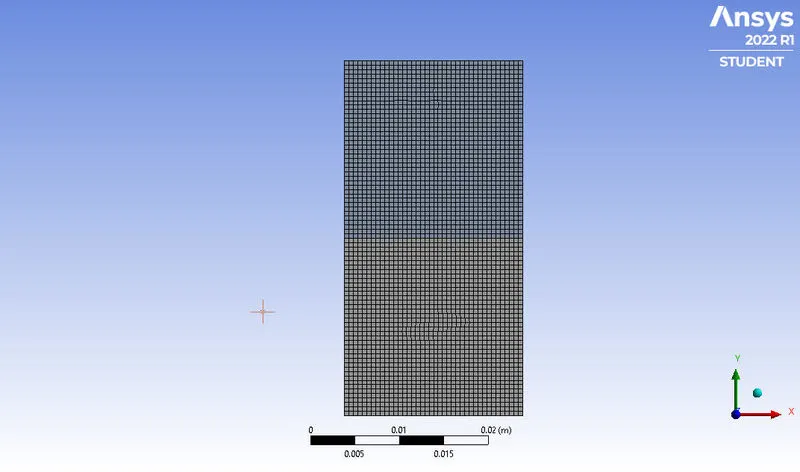
Total numbers of elements are 3200.
Setup:
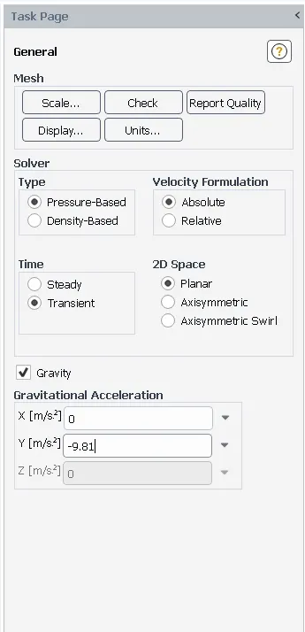
SOLVER TIME - TRANSIENT STATE
SOLVER TYPE - PRESSURE BASED
ENABLE GRAVITY AND IN THE ANSYS FLUENY Y AXIS SHOWS UPWARD AND DOWNWARD DIRECTION SO FOR CONSIDERING THE GRAVITATIONAL EFFECTS PUT THE VALUE FOR Y AIS AS 9.81m/s^2.
Transient state over Steady-state for such simulations:
In RT instability, due to sudden collapse horizontal plane between dense and lighter fluid shock waves generated because of that bubbles and spike formation takes place which is obviously time-dependent. Hence, using a steady-state solver for such kind of simulations where we are more interested in knowing the flow field variables varies with respect to time will not work.
Naturally occurring R–T instabilities are quite common (e.g. in oceans, supernova and oil-trapping salt domes), but are hard to record because of their transient nature and fast (with the exception of salt domes) transition to mixing and turbulence. That\'s why we prefer to do transient simulation to steady-state simulation for such kind of problems.
> Energy eqautions are off and use laminar as viscous model we are using laminar as viscous model becuase velocity should be fairly slow for the simulation.
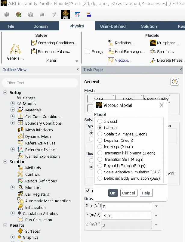
> Enable Multiphase model and select volume of fluid model where we have two eulerian phases where first phase reprasents the air and second phase reprasents the water and viceversa.
> Use implcit model.For the implicit model there is not any requirement for the calculation of the Courant number.
Physics > Model > Multiphase > select model as volume of fluid > select implicit as formulation > apply and close.
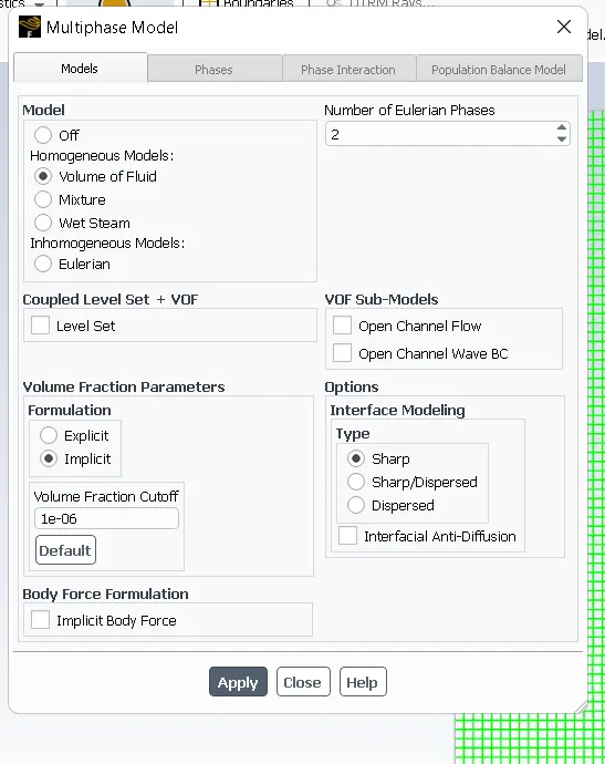
MULTIPHASE: Multiphse floe is simultaneous flow of material with diffrent mesh states or phases(liquid-gas)
It is a flow of materials with diffrent chemical properties but in the same state or phase(liquid-liquid)
VOLUME OF FLUID: Volume of fluid method is a surface tracking method.
It is designed to find out the position of interface between the two or more immiscible fluids.
The volume fraction of each fluid in each of cell throughout domain can be tracked by using this method.Single set of momentum equations is shown only by fluids.
In this method all the control volume must be filled with single phase or combination of phases.
Application of vof model include stratified flows,free surface flows, filling,sloshing,the motion of large bubble in liquid,the motion of liquid after a dam break,the prediction of jet breakup(surface tension) and the steady and unsteady tracking of liquid gas interface.
EXPLICIT SCHEME: It offers time accurate data, but timestep size has to be taken ensuring that the courant number is satiafied.
IMPLICIT SCHEME: It will offer the speed of the steady state but we need a time varrying solution.
> It is unconditionally stable( time step size is not a constraint) and is default scheme in ansys fluent.
> LIST THE PHASES:
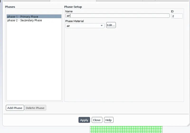
PHASES > PHASE 1 > PRIMARY PHASE > CHANGE NAME TO AIR
PHASE 2 > SECONDARY PHASE > CHANGE NAME TO WATER
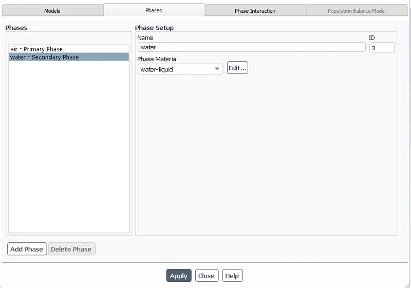
Material: For this setup use two materil one is air and another as water.
Add water from fluent database.
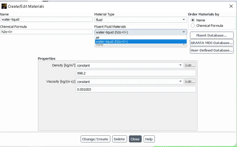
> Initialize the problem using standard initialization.
> Perform Patching
Patch > select water under the phase > select volume fraction as variable > select water surface > and give as 1 > patch
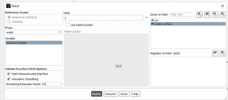
select fff surface > unselect water surface > give value as 0 > patch > close.
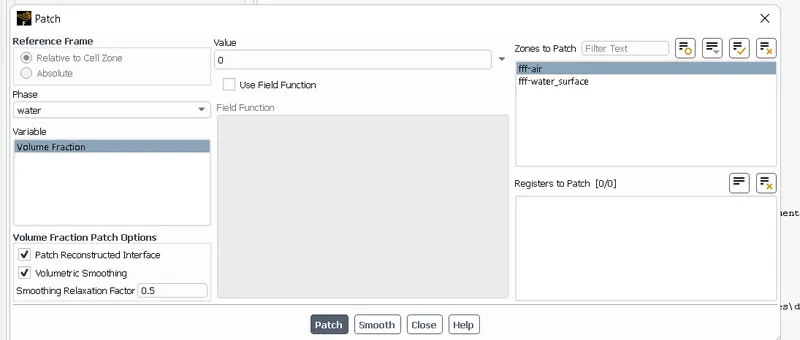
What is the meaning of patch?
When we have two phase the phases are actually reprasented by value "A" whnen the value of A is 1 it reprasent one phase it could be water or air and when A is 0 it reprasent another phase.
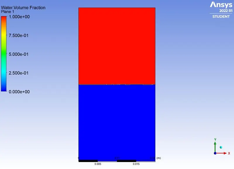
For example: When A equal to 1 we have water phase which when we initialize we want A=1 only at top because we required highier density fluid at top and A=0 at bottom so this means that your initialization process is correct.
Simply Patching is done for case setup that we required.
How do we make sure that initialization that we have done is setup correctly?
> For that we have to create contours.
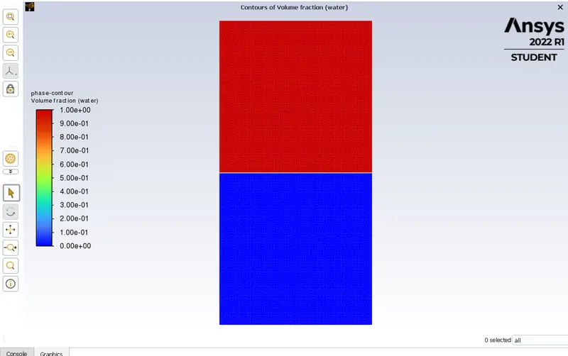
Post processing > contours > New > phases > Volume fraction > Water > select all > save and display.
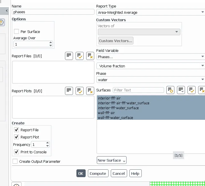
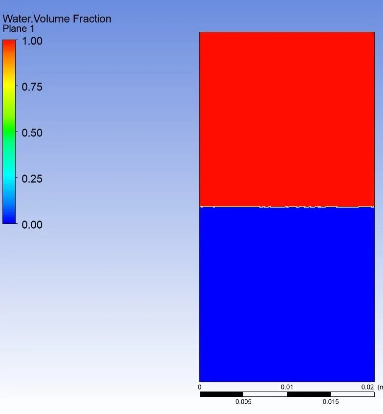
So it reprasents volume fraction of water which shows that volume of water at top is 1 and volume of water at bottom is zero,so this tells that setup is correct.
> Run the simulation for the time step size of 0.01.
and no. of steps used are 500.

> RESULTS:
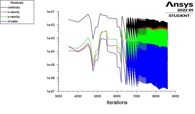
>Scaled residuals:
> Volume fraction contour:
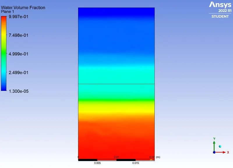
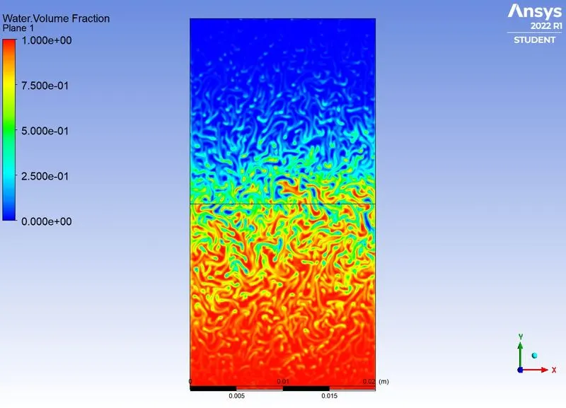
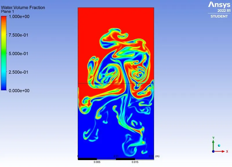
Water will come down and air will go up due to density difference.
> POST PROCESSING:
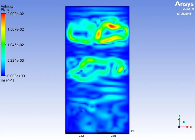
Velocity:
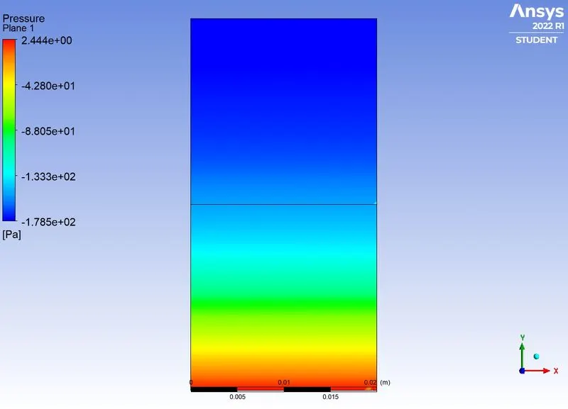
> Pressure:
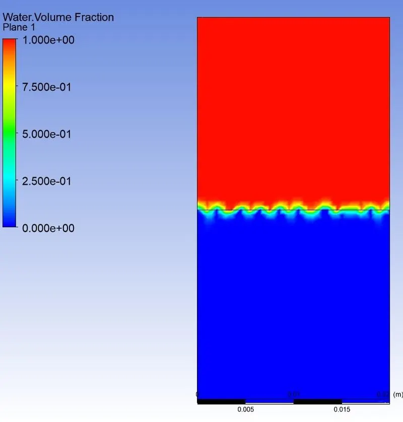
> Water volume fraction for diifrent time steps:
For time step 0.02seconds.
> For time step size of 0.6 seconds
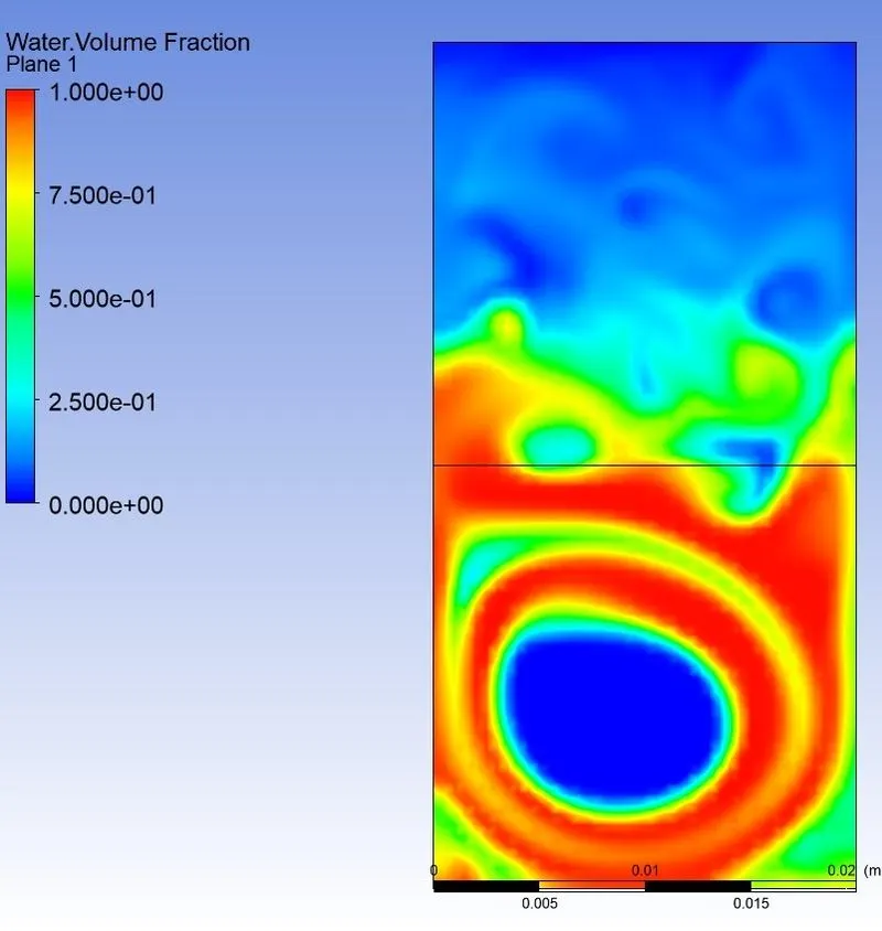
> For time step size of 1 second
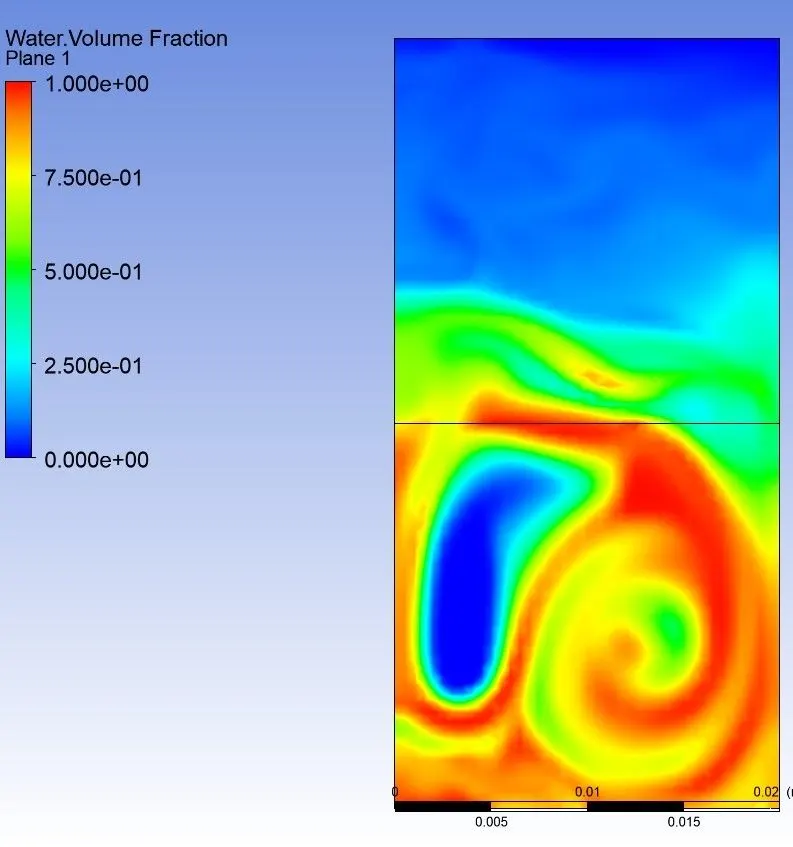
> For time step size of 2 seconds
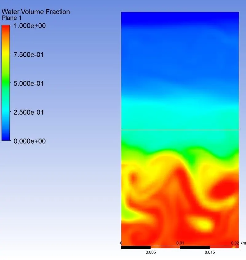
> For time step size of 4 seconds
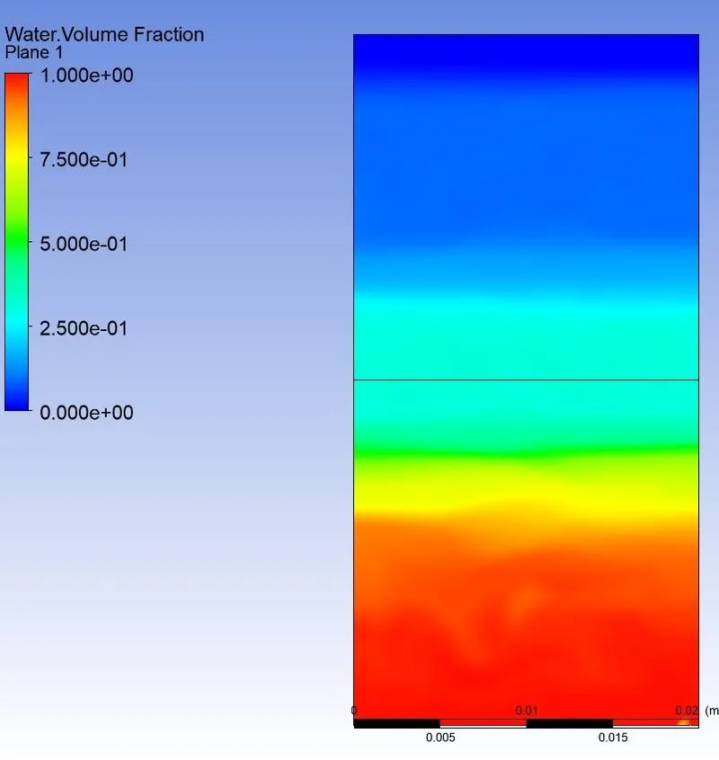
VIDEO ANIMATION FOR WATER VOLUME FRACTION:
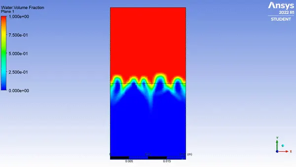
CASE 2 :
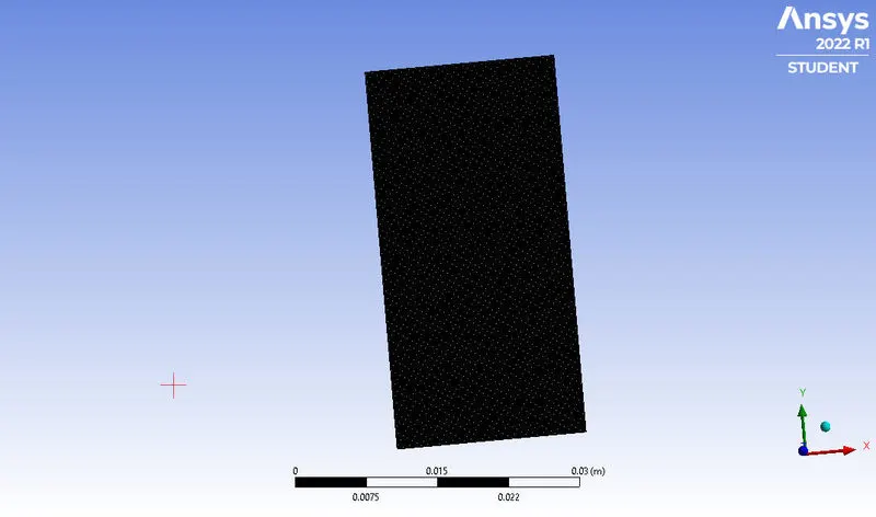
MESHING:
meshing with element size of 0.1mm
total no. of elements are 8000.
Setup:
|
|||||||||||||||||||||
| time step size as 0.001 | |||||||||||||||||||||
| No of steps as 1500 |
Results:
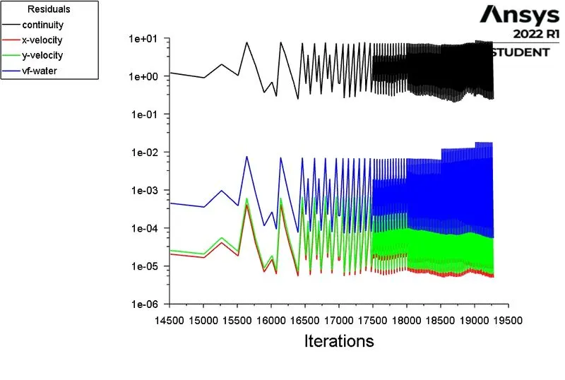
Scaled residuals:
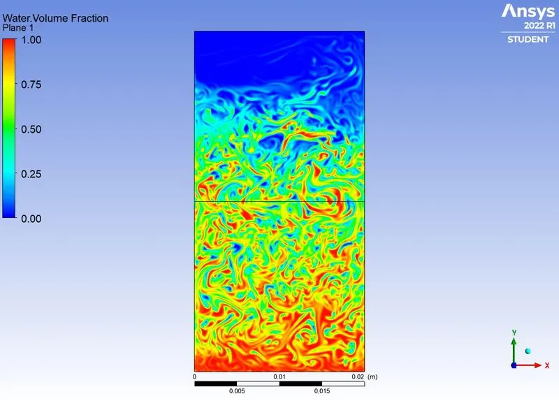
Water volume fraction:
> Post processing:
> water volume fraction for diffrent time step
> water volume fraction for 0.02 seconds
> water volumr fraction for 0.4 seconds
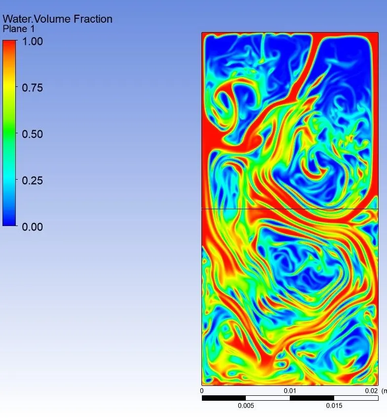
> water volume fraction for 0.6 seconds
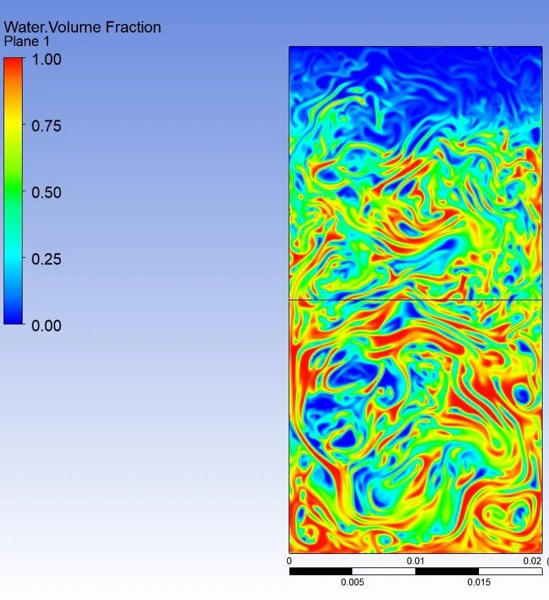
> water volume fraction for 0.8seconds
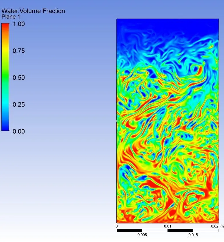
> water volume fraction for 1 second
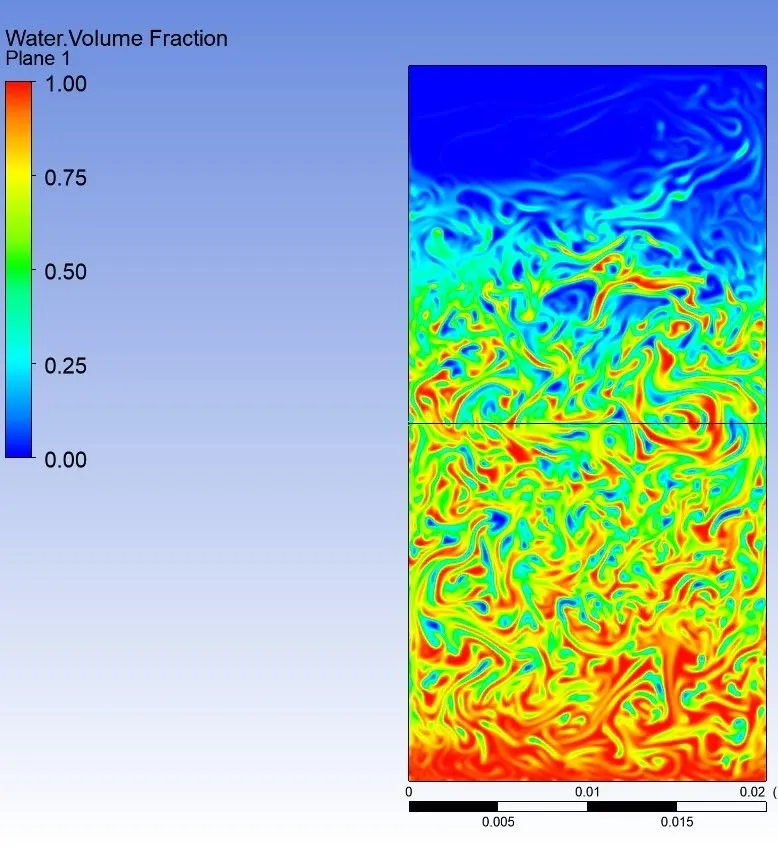
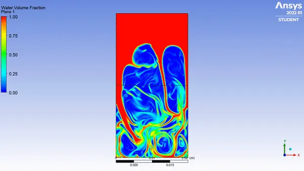
> ANIMATION FOR WATER VOLUME FRACTION:
Case 3:
Meshing:
meshing with element size of 0.1mm
total no. of elements are 8000.
Setup:
| Solver type | Pressure based |
| Solver time | Transient state |
| Multiphase ( Volume of fluid) | ON |
| Energy | OFF |
| Viscous model | Laminar |
| Material | User defined material(density= 400kg/m^3, kinematic viscocity as 0.001kg/ms) and Water |
| Primary phase | user defined material |
| Secondary phase | Water |
| Method | coupled |
| Patching | Done |
Time step size is 0.001
Number of steps are 3200
Results:
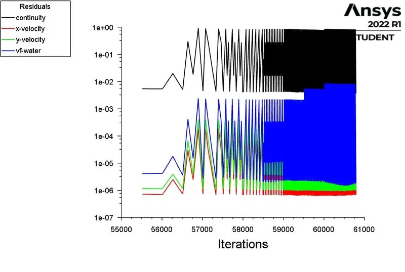
> Scaled Residuals:
> Water volume fraction:
> POST PROCESSING:
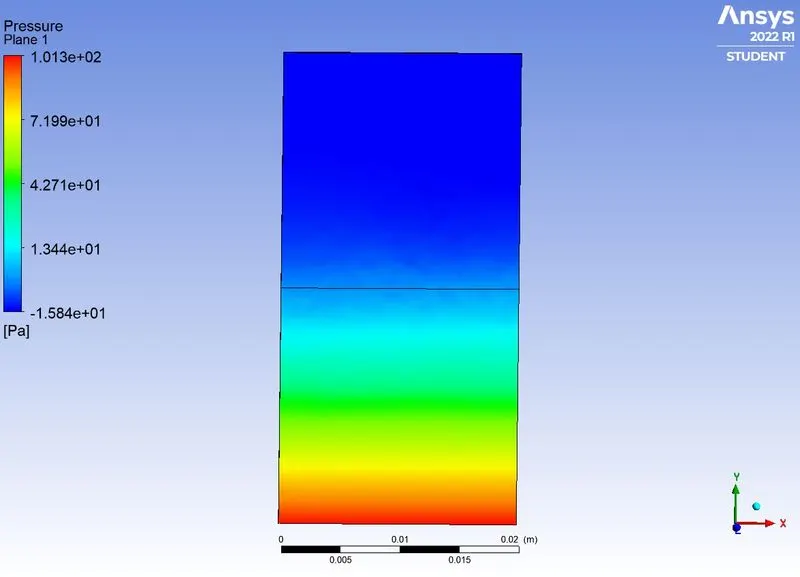
> Pressure:
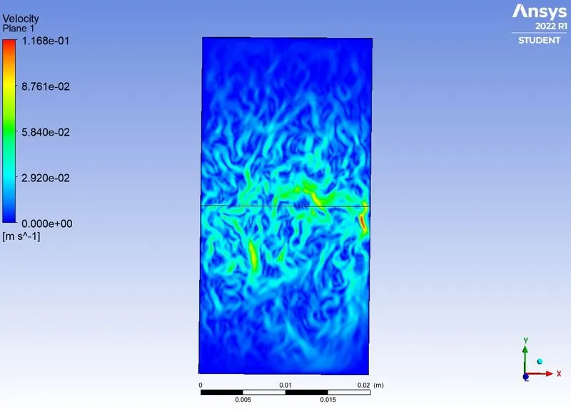
> Velocity:
> Water volume fraction at diffrent Time zones:
> water volume fraction at 0.02 seconds:
> water volume fraction at 0.50seconds:
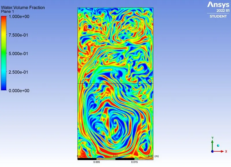
> Water volume fraction at 1 seconds:
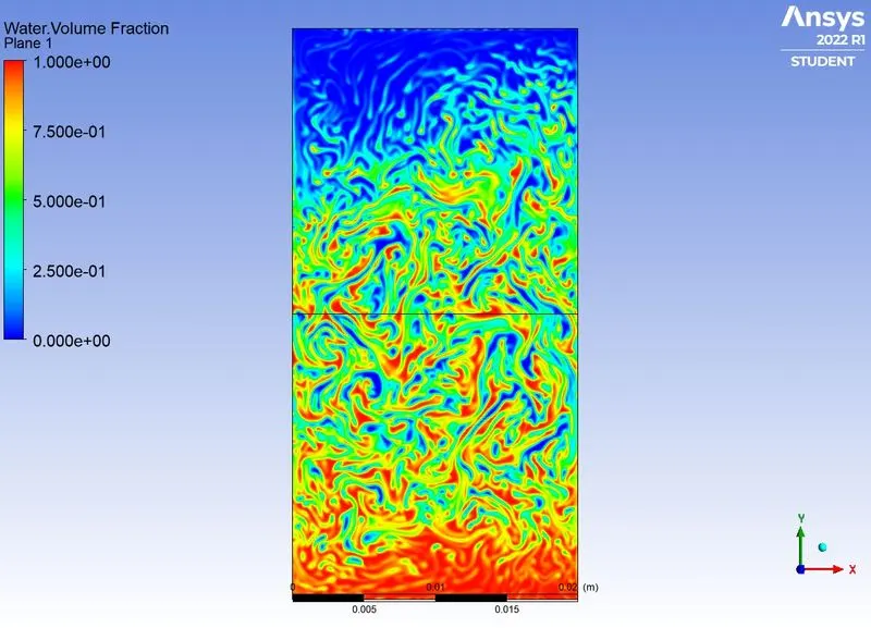
> water volume fraction at 2 seconds:
> water volume fraction at 3 seconds:
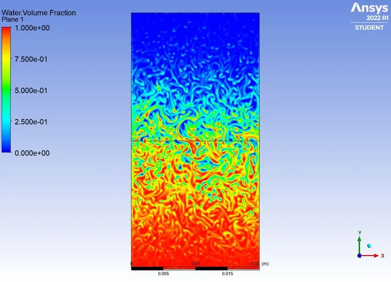
> water volume fraction at 3.2 seconds:
> VIDEO ANIMATION:
>
Atwood no:
It is a dimensionless no in fluid dynamicsused in the study of hydrodynamics instabilities in density stratified field.
Atwood no.close to 0, means RT instability flows take the form of symmetric “fingers” of fluid.
for Atwood number close to 1, the much lighter fluid “below” the heavier fluid takes the form of larger bubble-like plumes.
A=ρ1-ρ2ρ1+ρ2">A=(ρ1−ρ2)/(ρ1+ρ2)
where, rho1 is the density of heavier fluid and rho2 is the density of lighter fluid.
Here, in this case water is considered as heavier fluid and Air is considered as lighter fluid.
Densities:
rho1= 998.2 kg/m3 (Density of Water)
rho2= 1.225 kg/m3 (Density of Air)
A=998.2-1.225998.2+1.225">A=(998.2−1.225)/(998.2+1.225)
Here, the value for Atwood number in the above case we found is 0.997548.
>`Hence from the value, we can say that RT instability, in this case causes the formation of bubbles and spike.
> Atwood no close to 1 indicates the bubble formation, and value close to 0 indicates wake like formation without any bubble.
> Small density differences, At<0.1, up-welling (‘bubble’) and down-welling (‘spike’) disturbances form a symmetrical mixing region that expands away from the initial position of the density interface.
Asymmetries in the penetration of rising bubbles and falling spikes are readily apparent when At>0.5. As the Atwood number increases, the spike penetration is greater than that of the bubble owing to a narrowing of the spike, and a consequent reduction of drag on the head of the spike.
At=1, both bubble and spike portion approaches constant velocity when fluid densities are similar.
> CONCLUSION
>The finer the mesh, the more correct the observation of bubble formation can be captured. coarse mesh achieves stability or we can say that heavier fluid settled in very less period of time.
> With increase in mesh refinement, the computational time increases.
> The Atwood number validates the CFD simulation as it is observed. In case of water and air mixing, bubble formation takes place, whereas for the other case no bubble takes place.
> Incorrect or large time step leads to \'Floating point exception\' error because the solver detects arithmetic operation which can not compute. It results in a sudden rise in residuals during runtime. This depends on problem to problem.
> Finner mesh is quite useful in terms of capturing data during the process but it will certainly take more time to get to the stability.
> We can observe bubbles and spikes in all simulation but finner mesh makes visualization better obvious.