Week 5 - Rayleigh Taylor Instability

RAYLEIGH TAYLOR INSTABILITY

• The instability of a heavier fluid layer supported by a light one is generally known as Rayleigh-Taylor (RT) instability. It can occur under gravity and, equivalently, under an acceleration of the fluid system in the direction toward the denser fluid. A simple example may illustrate typical evolution times for the overturn of ordinary liquids under the effect of the earth’s gravity. Assuming an acceleration a=9.8m/s² and a perturbation wavelength λ = 1cm, the classical e-folding time τ = √ λ / √2 of the free-surface RT instability would be 0.013s. Even if an unstable equilibrium would be established, the instability evolution would be too fast for direct observation. However, the typical finger-like flow patterns can be nicely modeled, for instance, by Hele-Shaw cells consisting of thin sheets of viscous fluid inside the gap between two parallel glass plates.
• Because of the transient nature of RT instabilities in common situations, its physical significance may have escaped for a long time. Experimental observations of RT instabilities have only started with the work of Taylor and Lewis about forty years ago, although Rayleigh’s theoretical analysis dates back to the end of the last century. At present, a number of laboratory experiments with accelerated liquid have been reported that illustrate the instability evolution under various circumstances.
• The experiments conducted by Lewis have shown three subsequent stages in the evolution of an unstable air-water interface. The initial phase of exponential growth is followed, first, by a transition phase of bubble formation and then by an asymptotic stage of rising air columns. One should clearly distinguish between the instability problem, related to the initial phase, and the mixing problem, related to the asymptotic phase. In the stability problem, one is mainly concerned with the modification of instability growth rates by various physical effects. In contrast, the mixing problem is addressed to the penetration of perturbation fronts through the liquid.
• The instability evolution between fluid layers of nearly the same density has been studied experimentally by Allred and Blount and by Ratafia. The density dependence can be expressed by the so-called Atwood number leading to appreciably lower growth rates for fluids with nearly equal densities. Moreover, the nonlinear evolution of the interface appears more symmetric, showing mushroom-like flow patterns in both fluids.
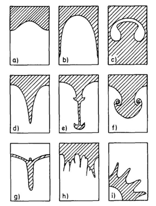
• An overview on characteristic flow patterns in the evolution of RT instabilities is given by the schematic drawings shown below. In this figure, the heavy (light) fluid is represented by shaded (unshaded) regions and the kinematical acceleration is directed vertically upward in (a-h) or radially inward in (i). Normal mode perturbations of the horizontal equilibrium surface give rise to sinusoidal surface modulations as represented in (a). The fluid interchange decreases the potential energy content of the system which is the cause of instability. The further upward motion of the lighter fluid assumes the form of rising gas bubbles with an approximately steady shape as illustrated in (b). For comparison, the evolution of a closed, initially spherical bubble is also shown in (c). These horseshoe-like deformations are based on incompressible inviscid fluid dynamics. Experimental observations of underwater bubbles have also indicated the formation of a turbulent wake. Typical feature of the falling heavy fluid are represented in (d-g). In a low-density gas, the fluid particles can closely approach the stage of free fall. A corresponding contraction of the downward flow gives rise to needle-shaped spikes as shown in (d). when the flow resistance of the lighter fluid becomes important as in (e), broadening oof the spike tips is observed along with the formation of mushroom-like vortex motions. These additional structures are commonly attributed to secondary shear flow instabilities. The pronounced differences between bubble and spikes disappear for fluids with nearly equal densities. Corresponding bubble-spike can be recognized in (f). Antispikes, of the form shown in (g), have been observed in fluid simulations at the stable rear side of an accelerated thin foil. The advantage stage of intermixing give rise to much more complicated patterns as illustrated in (h). RT instabilities are also often encountered in spherical geometries. For instance, implosions of inertial confinement fusion pellets are subject to outside surface instabilities during acceleration and to inside cavity instabilities during deceleration.

                                                                    

• Over the past decades it also become obvious that RT instabilities would play an important role in many different fields. Their control is of vital interest for a number of technological applications, in particular in inertial confinement fusion (ICF) devices. In geophysics, where some ionospheric phenomena, known as equatorial spread F bubbles, have been explained in the RT context. In astrophysics, certain chain-like globules in the interstellar medium show close resemblance with RT flow patterns. it is therefore believed that RT instabilities can occur in accelerated gas clouds, driven for instance by new-born stars or supernova events.

 RITCHMYER-MESHKOV INSTABILITY

• Richtmyer-Meshkov instability arises when a shock wave interacts with an interface separating two different fluids. It combines compressible phenomena, such as shock interaction and refraction, with hydrodynamic instability, including nonlinear growth and subsequent transition to turbulence, across a wide range of Mach numbers.
• Some examples are Supersonic combustion in a scramjet, Combustion, supernova, hypersonic air-breathing engines.
• In case of combustion, Instability begins with a very small amplitude perturbations which initially grow linearly with respect to time. The instability can be considered the implusive-acceleration limit of the Rayleigh Taylor Instability. During the implosion of an inertia confinement fusion target , the hot shell material surrounding the cold D-T fuel layer is shock accelerated. Such instability is visualized in Magnetic target fusion.

PLATEAU–RAYLEIGH INSTABILITY

• The Plateau–Rayleigh instability, often just called the Rayleigh instability, explains why and how a falling stream of fluid breaks up into smaller packets with the same volume but less surface area. This fluid instability is exploited in the design of a particular type of ink jet technology whereby a jet of liquid is perturbed into a steady stream of droplets.

KELVIN–HELMHOLTZ INSTABILITY

• Kelvin-Helmholtz studied the dynamics of two fluids of different densities subjected to a small disturbance such as wave was introduced at the boundary connecting both the fluids. This phenomena is mostly responsible for nature’s basic structures. It can occur when there is velocity shear in a single continuous fluid, or where there is a velocity difference across the interface between two fluids. Examples: wind blowing over water, clouds, the ocean, Saturn's bands, and the sun's corona 

DESCRETE BOLTZMAN MODEL

• Discrete Boltzmann model (DBM) is a type of coarse-grained mesoscale kinetic model derived from the Boltzmann equation. Physically, it is roughly equivalent to a hydrodynamic model supplemented by a coarse-grained model for the relevant thermodynamic non-equilibrium (TNE) behaviours. 
• It is developed to investigate the hydrodynamic and thermodynamic non-equilibrium effects in phase separation processes. Based on the thermodynamic non-equilibrium features, its estimates the deviation amplitude from the thermodynamic equilibrium.

BASELINE SIMULATION

GEOMETRY SETUP

• Open in space claim
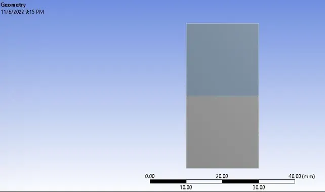
• Creating a square with a dimension of 20 x 20 mm and using the pull tool to creating the surface.
• After the surface is generated, then moving the generated component to a new component and named it as air. Now a new component that represents as water is designed.
• 
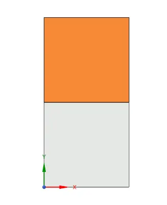
• After both the components are created and checked.
• In share topology option click to share.
• 

MESH

• After the geometry is created, now the next step is to generate the mesh.
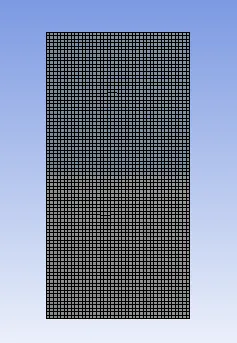
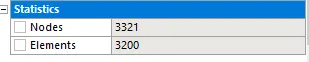
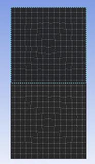
• Open the mesh, a baseline mesh is generated with an elemet size of 0.5mm.

 

SET UP OF PHYSICS

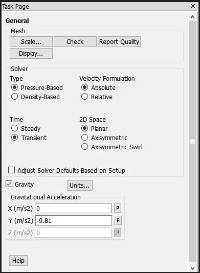
• In set up, after the geometry is loaded, perform check mesh using the check mesh option.
• Solver type   :  pressure based
• Time : Transient state
• Velocity formulation : absolute
• Enable the gravity option and giving a value of -9.81m/s^2(in negative y direction)
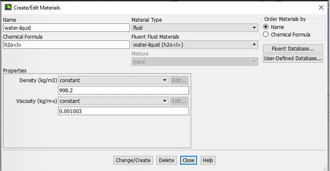
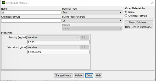
• Material  : Fluid 1   : Air
•                 Fluid 2  : Water
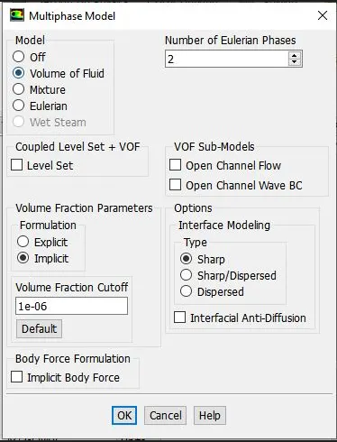
• In models enable the multiphase flows and in select VOF method.
• Number of Eulerian phases  : 2
• Formulation type : implicit
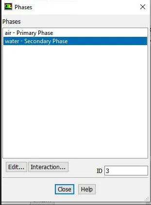
• In phases option, we selected two phases give names and selcect phase,for primary phase :change name as air and change phase material to air. For secondary phase :change name as water and change phase material to water.
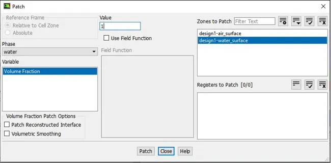
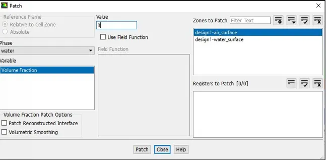
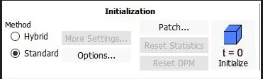
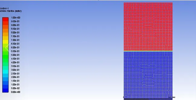
• Now we have to initialize first and then we do Hybrid initialization.Now, patch the value fraction value of 0 to air side and 1 to water side.
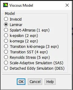
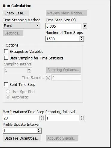
• The below images shows the above mentioned steps for setting up the physics.

RESULTS

CASE-1 (Baseline simulation)

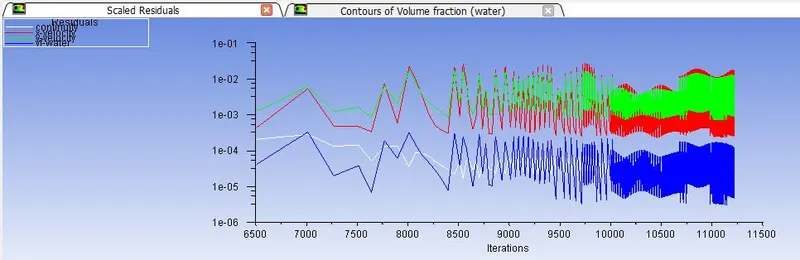
RESIDUALS

CONTOURS OF VOLUME FRACTION

FRAMES

CASE-2-REFINED MESH 

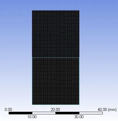
• Element size: 0.3
• Time step size: 0.005
• No of time step: 1000

MESH

 

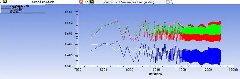
RESIDUALS

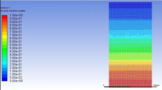
CONTOURS OF VOLUME FRACTION

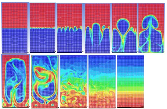
FRAMES

CASE-3-REFINED MESH 

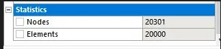
• Element size: 0.2
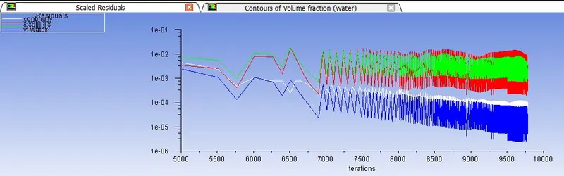
• Time step size: 0.005
• No of time step: 1000

MESH

RESIDUALS

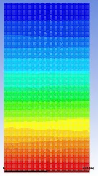
CONTOURS OF VOLUME FRACTION

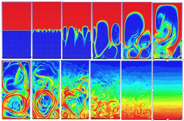
FRAMES

CASE-3-REFINED MESH WITH USER MATERIAL AND WATER.

• Element size: 0.1
• Time step size: 0.005
• No of time step: 1000

RESIDUALS

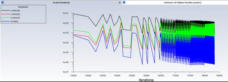
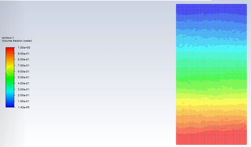
CONTOURS OF VOLUME FRACTION

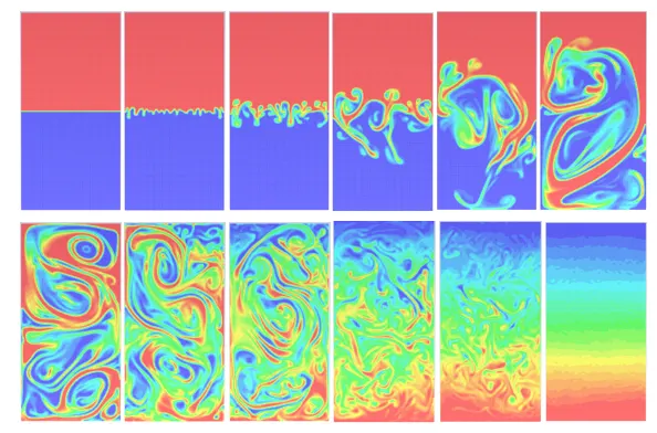
FRAMES

Atwood number.

• It is a dimensionless number in fluid dynamics, used in the study of hydrodynamic instabilitis in density stratified flows.
• It should gives the relationship between density of higher fluid and the density of lighter fluid.
• It should used in the study of Rayleigh Taylor instability.
• The Atwood number closes to 1 means the lighter fluid should below the heavier fluid takes the form of large bubble like plumes.
• For case-1, Atwood number for air and water equal to 0.9975. 

                  

• For case-1, Atwood number for user defined material and water equal to 0.4278. 

                   

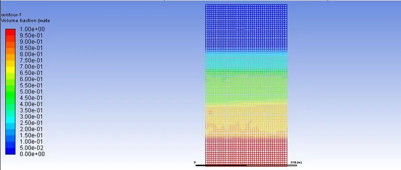
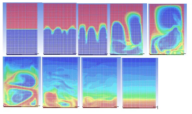
•  It is observed from the above simulations that air forms larger bubbles when water is burst down the air and forms large bubbles. Atwood number calculated in case -1 is 1 (approx.) and  case-2 is 0.42. Rayleigh Taylor instability shows three distinct stages which are  Linear stability ,  bubble formation and bubble merging and mixing.

 CONCLUSIONS

•  Here transient analysis is preffered instead of steady state analysis, because here we are interested in real time changes at the fluid interface.  it is also a time marching solution, expect more accuracy from transient simulation for which Transient simuation is the ideal setup to run the calculation for Rayleigh Taylor Instability.
• From the above computational analysis, its been evident that more we refine the mesh, the more the simulation gets smoother in irregularities which takes place at the interface of the two fluids.
• Finer mesh shows formation of bubbles and vortices, the higher density fluid replaces the lower density thus the formation of bubbles and vortices takes place and travel toward to the upper region with respect to time.