Week 5 - Rayleigh Taylor Instability
Aim: To conduct the Rayleigh Taylor CFD simulation.
Objective:
What are some practical CFD models that have been based on the mathematical analysis of Rayleigh Taylor waves? In your own words, explain how these mathematical models have been adapted for CFD calculations.
Perform the Rayleigh Taylor instability simulation for 2 different mesh sizes with the base mesh being 0.5 mm. Compare the results by showing the animations( Attach them from your google drive). Observe the differences in the animation and explain the effect of mesh size on the simulation. Also, explain why a steady-state approach might not be suitable for these simulations. [Choose Air and Water for this simulation]
For refined mesh, run one more simulation with water and user-defined material(density = 400 kg/m3, viscosity = 0.001 kg/m-s).
Define the Atwood Number. Find out the Atwood number for both cases and explain how the variation in the Atwood number in the above two cases affects the behavior of the instability.
Theory:
Rayleigh Taylor Instability (RTI) is a phenomenon that occurs at the interface of fluids of different densities wherein the lighter fluid pushes the heavier fluid due to the density difference. It is a dynamic process wherein the system tries to reduce its combined potential energy. Initially, the system is in a state of hydrostatic equilibrium, in which the heavier fluid(ex: water) sits atop a lighter fluid(ex: air) in a constant gravitational field. As the RTI develops, the initial perturbations progress from a linear growth phase, eventually developing "plumes" flowing upwards(in the gravitational buoyancy sense) and "spikes" falling downwards. In the linear phase, equations can be linearized and the amplitude of perturbations is growing exponentially with time. In the non-linear phase, the perturbation amplitude is too large for the non-linear terms to be neglected. In general, the density disparity between the fluids determines the structure of the subsequent non-linear RT instability flows (assuming other variables such as surface tension and viscosity are negligible here). Examples include supernovas, water suspended atop oil, and mushroom clouds formed due to volcanic eruptions.
There are some practical CFD models that have been based on the mathematical analysis of Rayleigh Taylor waves:
Kelvin–Helmholtz instability
The Kelvin–Helmholtz instability (after Lord Kelvin and Hermann Von Helmholtz) can occur when there is velocity shear in a single continuous fluid, or where there is a velocity difference across the interface between two fluids. An example is a wind blowing over water: The instability manifests in waves on the water's surface. More generally, clouds, the ocean, Saturn\'s bands, Jupiter\'s Red Spot, and the sun\'s corona show this instability. The theory predicts the onset of instability and transition to turbulent flow in fluids of different densities moving at various speeds. Helmholtz studied the dynamics of two fluids of different densities when a small disturbance, such as a wave, was introduced at the boundary connecting the fluids. For a continuously varying distribution of density and velocity (with the lighter layers uppermost, so that the fluid is RT-Stable), the dynamics of the KH instability is described by the Taylor-Goldstein equation and its onset is given by the Richardson number Ri. Typically the layer is unstable for Ri<0.25. These effects are common in cloud layers. The study of this instability is applicable in plasma physics, for example in inertial confinement fusion and the plasma - berryllium interface.
Numerically, the KH instability is simulated in a temporal or a spatial approach. In the temporal approach, experimenters consider the flow in a periodic (cyclic) box \"moving\" at mean speed (absolute instability). In the spatial approach, experimenters simulate a lab experiment with natural inlet and outlet conditions (convective instability).
Richtmyer–Meshkov instability
The Richtmyer–Meshkov instability (RMI) occurs when two fluids of different densities are impulsively accelerated. Normally this is by the passage of a shock wave. The development of the instability begins with small amplitude perturbations which initially grow linearly with time. This is followed by a nonlinear regime with bubbles appearing in the case of a light fluid penetrating a heavy fluid, and with spikes appearing in the case of a heavy fluid penetrating a light fluid. A chaotic regime eventually is reached and the two fluids mix. This instability can be considered the impulsive-acceleration limit of the Rayleigh-Taylor instability. During the implosion of an inertial confinement fusion target, the hot shell material surrounding the cold D-T fuel layer is shock-accelerated. This instability is also seen in Magnetized Target Fusion. Mixing of the shell material and fuel is not desired and efforts are made to minimize any tiny imperfections or irregularities which will be magnified by RMI.
Supersonic combustion in a Scramjet may benefit from RMI as the fuel-oxidants interface is enhanced by the breakup of the fuel into finer droplets. Also, studies of deflagration to detonation transition (DDT) processes show that RMI-induced flame acceleration can result in detonation.
Plateau–Rayleigh instability
The Plateau–Rayleigh instability, often just called the Rayleigh instability, explains why and how a falling stream of fluid breaks up into smaller packets with the same volume but less surface area. It is related to the Rayleigh-Taylor instability and is part of a greater branch of fluid dynamics concerned with fluid thread breakup. This fluid instability is exploited in the design of a particular type of inkjet technology whereby a jet of liquid is perturbed into a steady stream of droplets. The driving force of the Plateau–Rayleigh instability is that liquids, by virtue of their surface tensions, tend to minimize their surface area. A considerable amount of work has been done recently on the final pinching profile by attacking it with self-similar solutions.
SPH method(Smoother particle hydrodynamics)
Smoothed-particle hydrodynamics (SPH) is a computational method used for simulating the mechanics of continuum media, such as solid mechanics and fluid flows. Smoothed-particle hydrodynamics is being increasingly used to model fluid motion as well. This is due to several benefits over traditional grid-based techniques. First, SPH guarantees the conservation of mass without extra computation since the particles themselves represent mass. Second, SPH computes pressure from weighted contributions of neighboring particles rather than by solving linear systems of equations. Finally, unlike grid-based techniques, which must track fluid boundaries, SPH creates a free surface for two-phase interacting fluids directly since the particles represent the denser fluid and space represents the lighter fluid.
Single-fluid model
A typical approach used for the analysis of two-phase flows is a mixture model, i.e. the individual fluid phases are assumed to behave as a flowing mixture described in terms of the mixture properties. The applied single-fluid model is a five-equation model consisting of the mass, momentum, and energy equations for a vapor/liquid mixture, and two equations describing the formation and growth of the liquid phase.
Two-fluid model
In the two-fluid model, separate sets of the governing equation for the vapor and liquid phases have been used. The interaction between the droplets and the heat exchange between the liquid phase and the solid boundary is not modeled here as well. Additionally, the velocity slip between the vapor and the liquid phase is in this model taken into account.
Turbulence model
Turbulence models are needed to predict the average mixing behavior inflows that are on average one- or two-dimensional. The approach to the construction of the tile turbulence model is guided by experimental behavior. The equations governing turbulent flows can only be solved directly for simple cases of flow. For most real-life turbulent flows, CFD simulations use turbulent models to predict the evolution of turbulence. These turbulence models are simplified constitutive equations that predict the statistical evolution of turbulent flows.
Simulation:
In this project, we consider 3 different cases in which 2 cases are based on the type of MESHING and the other is with user-defined materials.
The idea is, the dense fluid will be at the top and lighter fluid will be at the bottom and due to gravity, there will be instability at their interface, which is going to be calculated by using VOF multiphase method in ANSYS Fluent.
Water suspended a top oil is an everyday example of Rayleigh–Taylor instability, and it can be modeled by two completely plane-parallel layers of immiscible fluid, the denser on top of the less dense one, and both subject to the Earth\'s gravity. The equilibrium here is unstable to any perturbations or disturbances of the interface: if a parcel of heavier fluid is displaced downward with an equal volume of lighter fluid displaced upwards, the potential energy of the configuration is lower than the initial state. Thus the disturbance will grow and lead to a further release of potential energy, as the more dense material moves down under the (effective) gravitational field, and the less dense material is further displaced upwards.
In the below simulations fluids used are air and water with densities of 1.225 & 998.2kg/m^3. The method we are using is the Implicit method & we are using a volume of fluid method. There are three cases in the simulation in which above mentioned are kept constant and mesh sizes will be varied.
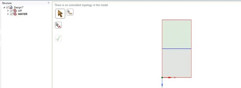
For our project, simply we consider a simple 2D geometry in which, We draw 2 squares one above the other with a length of 0.02 m. Then name the below square as air and the above square as water in 2 different components. And share the topology for a perfect intersection between both surfaces.
We consider 2 materials air and water placing one above the other and seeing the effect of gravity acting on them.
Step 1: GEOMETRY
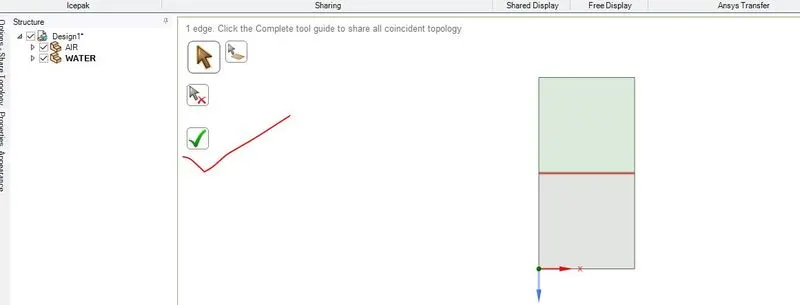
Firstly, the fluid flow fluent was dragged into the main operating window, then the space claim was opened, and after that, a sketch was created on the X-Y plane (x-horizontal axis) (y- vertical axis). The rectangle was created on the sketching module with 20x20mm dimension and the surface was created from that sketch, It moved into a new component Namely Air. Again, a new component is created under this secondly created component as water with the same dimension as shown above. And surface was extracted from that sketch.
Now for these two surfaces, we have to share topology so that we can generate a conformal mesh, in the meshing module. (Go to ) only a single edge was shared from the surface which is connecting both components.
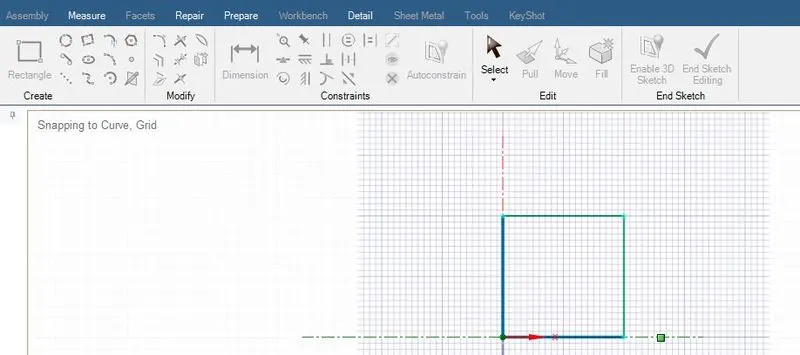
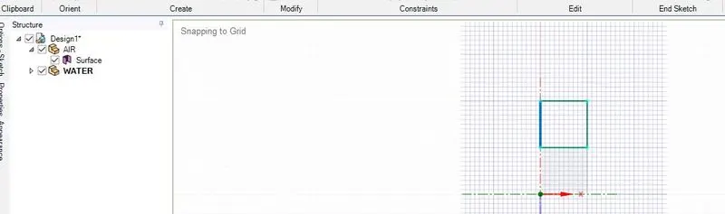
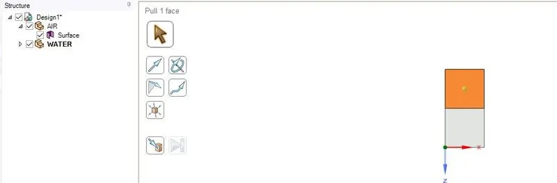
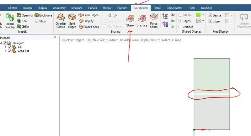
Step 2: Meshing
After the geometry preparation meshing was opened, here only meshing is an important parameter, and in this challenge, we have to carry out the instability behavior for three mesh sizes, so for the other two cases only the meshing size was modified,
For the first case, I took 0.5 mm mesh.
For second case = 0.3 mm
For third case = 0.1 mm
Considering all cases only the mesh size differed and the rest of the settings and boundary conditions are the same. considering the fluent setting also.
After meshing the fluent was opened, and the meshing was imported into the graphical window. Then I performed a mesh check operation.
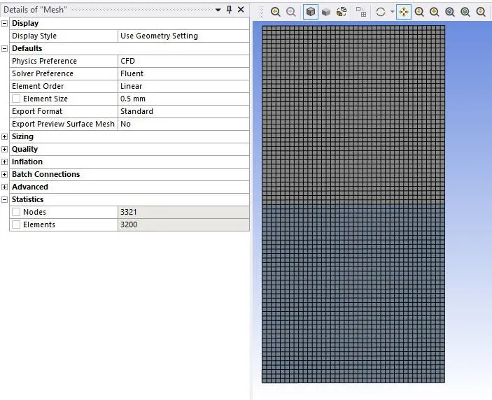
Case 1:
Element size:0.5 mm
No of Nodes: 3321
No of Elements:3200
Generated Mesh with the element size 0.5 mm
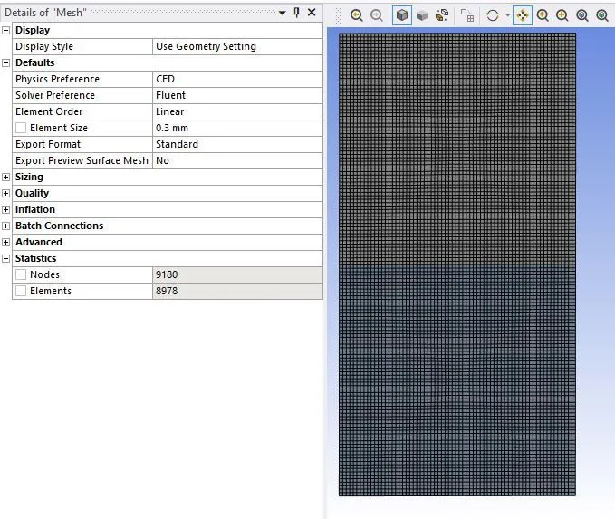
Case 2:
Element size:0.3 mm
No of Nodes: 9180
No of Elements: 8978
Generated Mesh with the element size 0.3 mm
Case 3:
Element size:0.1 mm
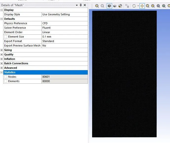
No of Nodes: 80601
No of Elements: 80000
Generated Mesh with the element size 0.1 mm
Step 3: Solver setting
Solver: Pressure-based
Time: Transient
Gravity: X = 0 m/s^2, Y = -9.81 m/s^2
Flow type: Laminar
Formulation: Implicit
Velocity formulation: Absolute,
2d space: planar
Multiphase Model type: Volume of fluid
After the general setting, the multi-phase model is selected as (volume of fluid method), and the other information is listed below in the image.
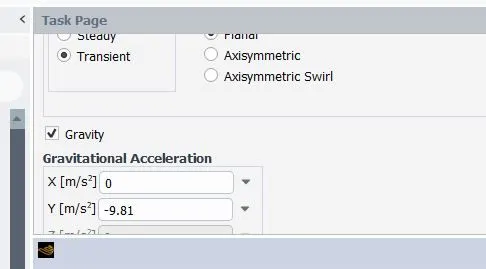
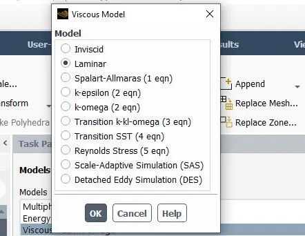
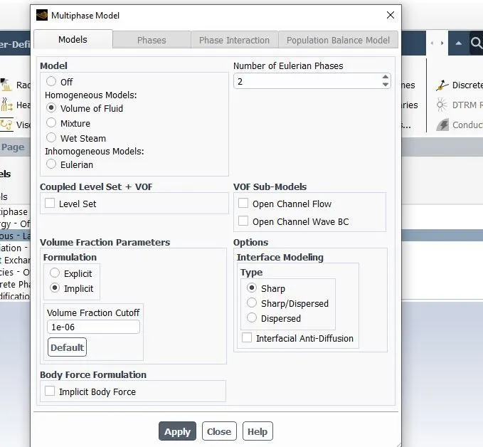
Material: Air and Water-Liquid
Setting fluids: Primary fluid as air, Secondary fluid as water-liquid
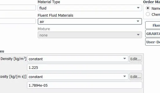
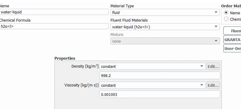
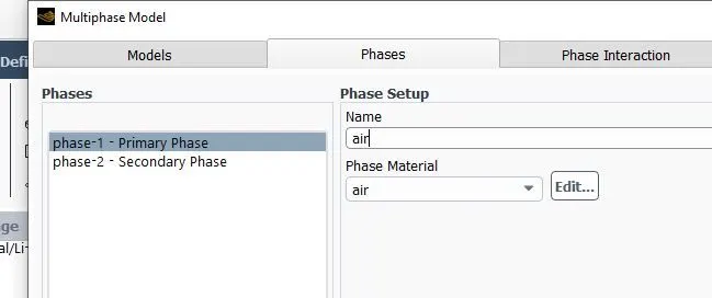
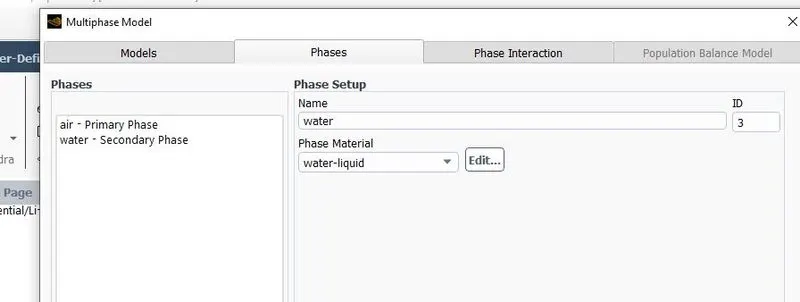
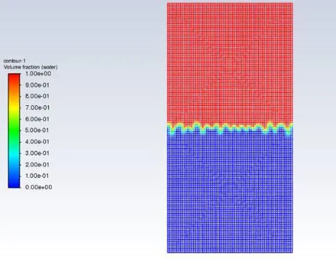
Then in the material panel, two material was imported just by coping from the fluent database. The material is Air and Water, then from the Phase menu, the list has to be modified from (list all phase menu). After renaming both phases in the listing, Standard initialization was done and the patching process was initiated to define that at the initial time step or at the start of the simulation the water is only upward, and in the lower portion only air must present. And both the fluids were sharing the same boundary. And mixing has to initiate after the first-time step is over.
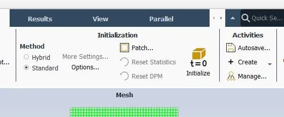
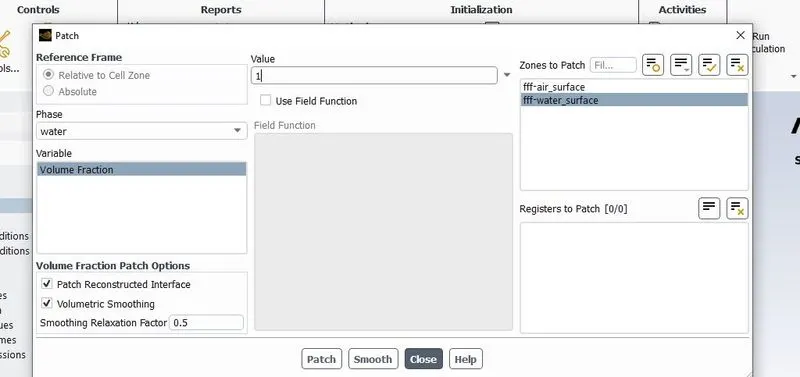
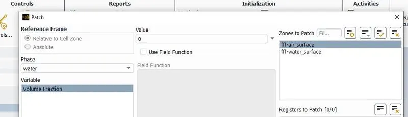
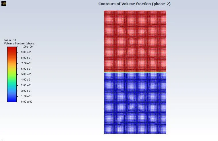
The bottom surface is air and the upper surface is water.
Calculation setting:
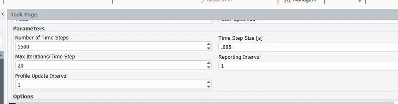
Time step = 0.005
No. of iteration = 1500
Results
In this way all the preprocessing and the basic boundary conditions are defined in space claim, meshing and Ansys Fluent. And the results of mixing fluid are carried out. The animation is attached to google drive.
Case 1:
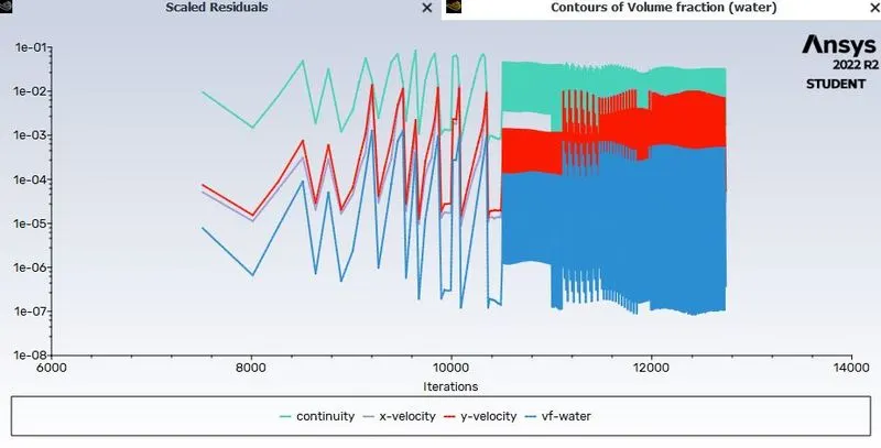
Scaled Residuals
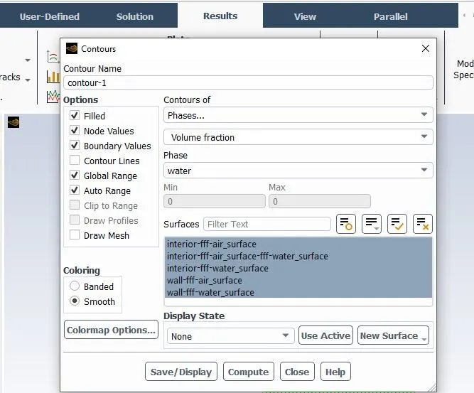
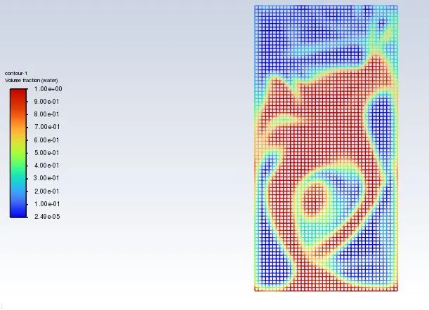
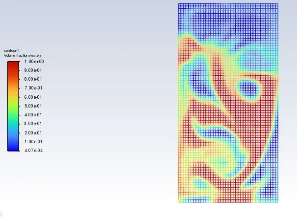
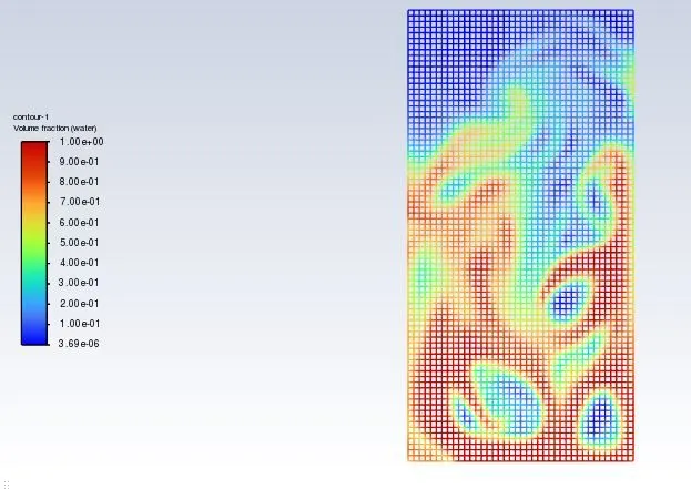
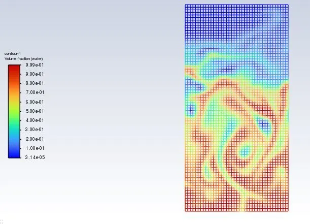
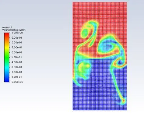
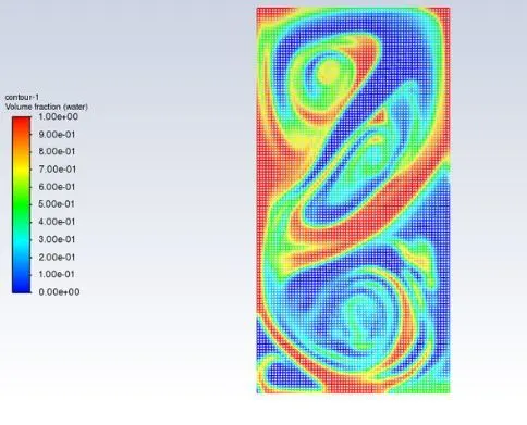
The contour of the volume fraction
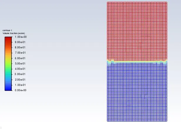
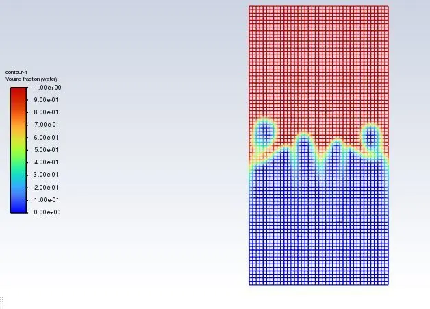
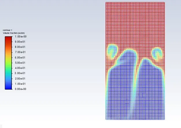
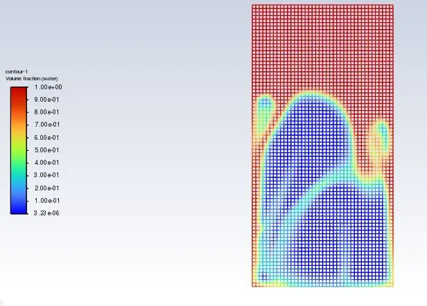
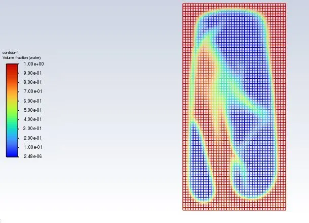
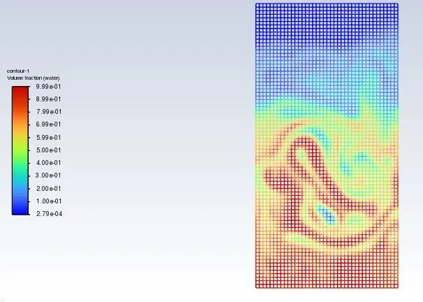
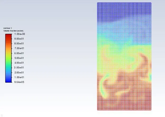
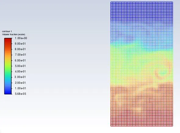
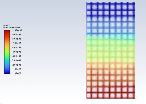
Animation
https://drive.google.com/file/d/1VqU1a_5_MVUayzz_0D0kt-t8qqBZNe1d/view?usp=share_link
Case 2:
Scaled Residuals
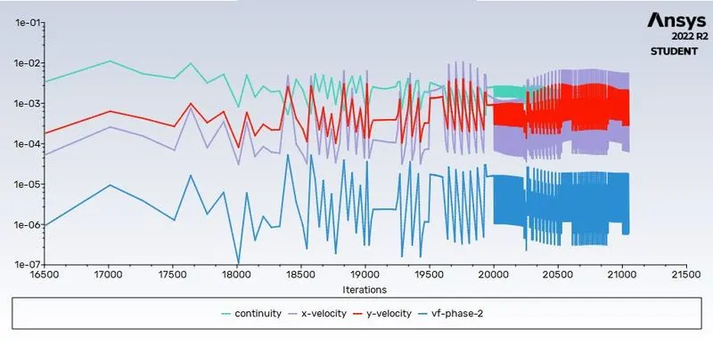
The contour of the volume fraction
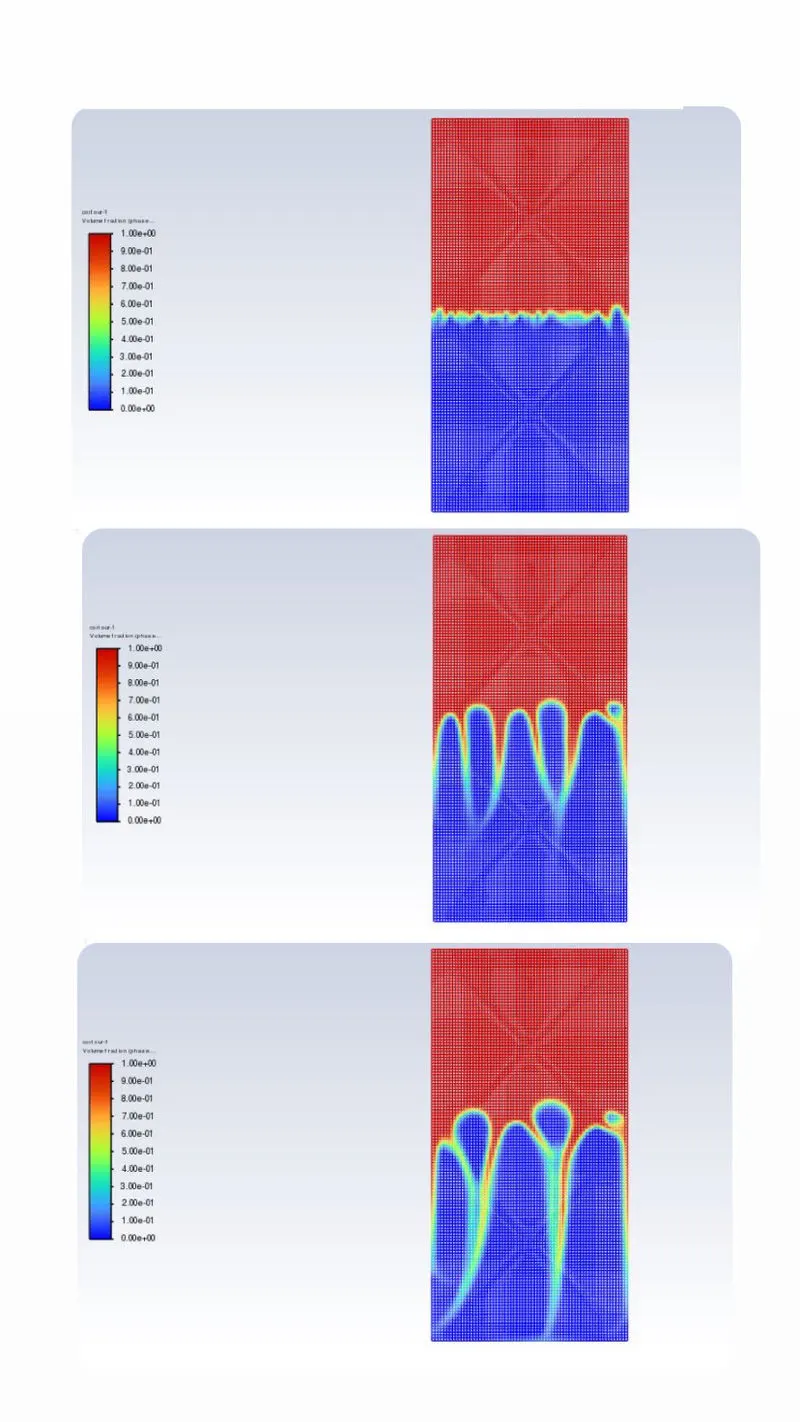
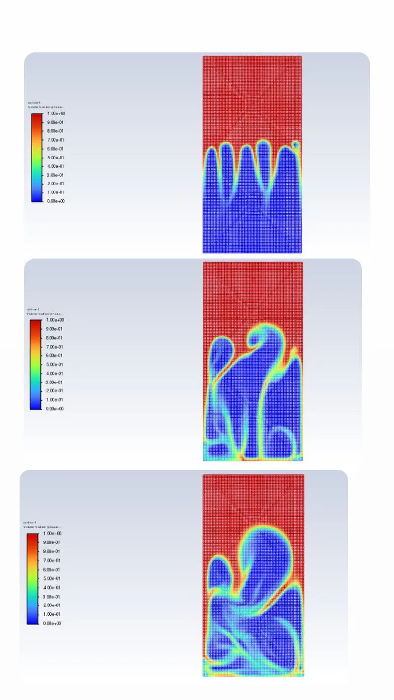
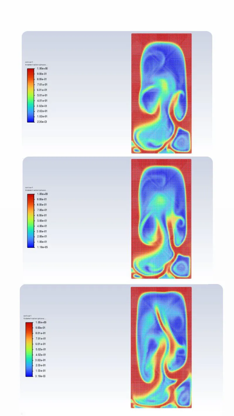
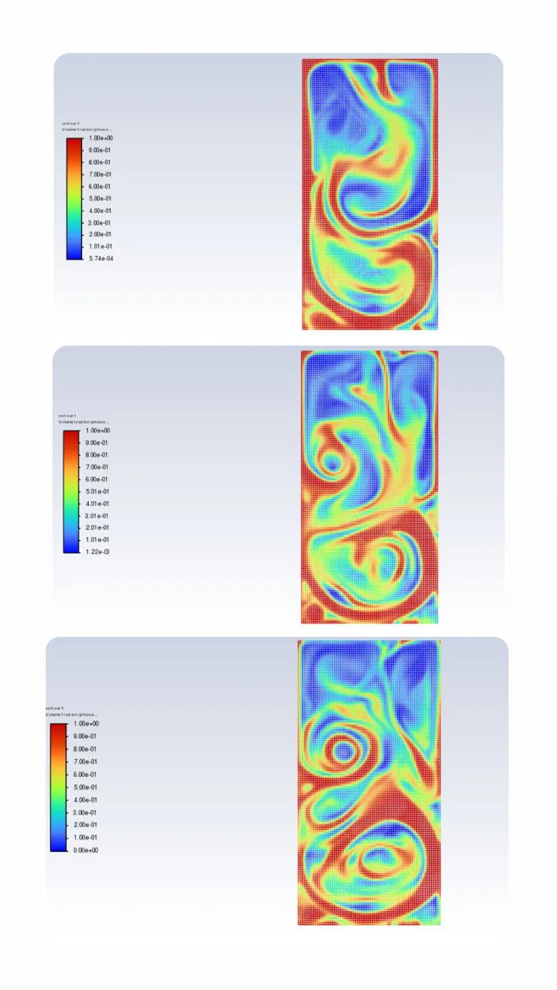
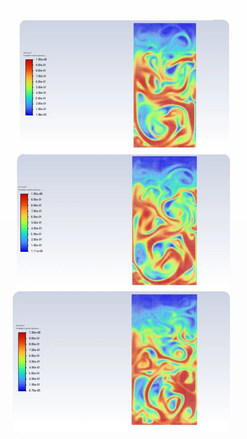
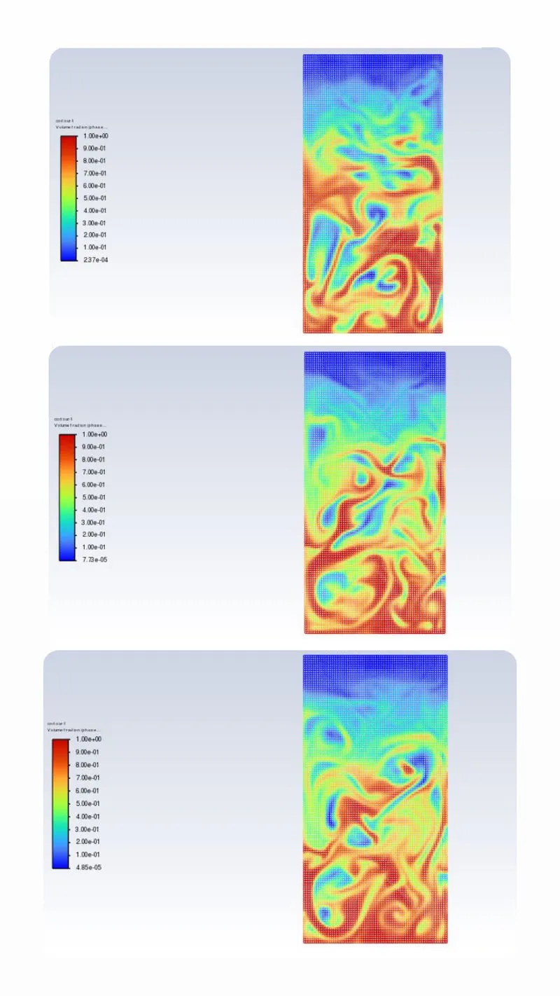
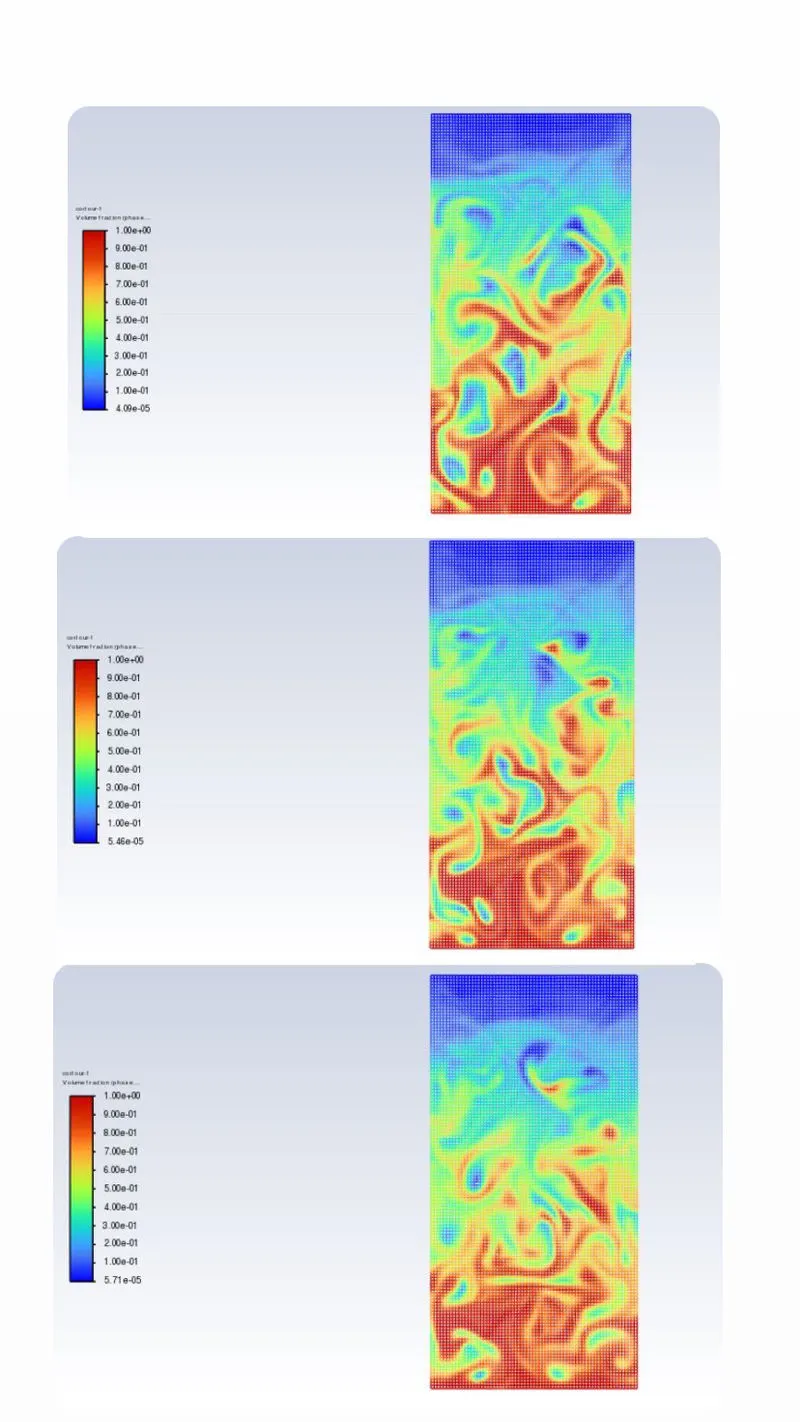
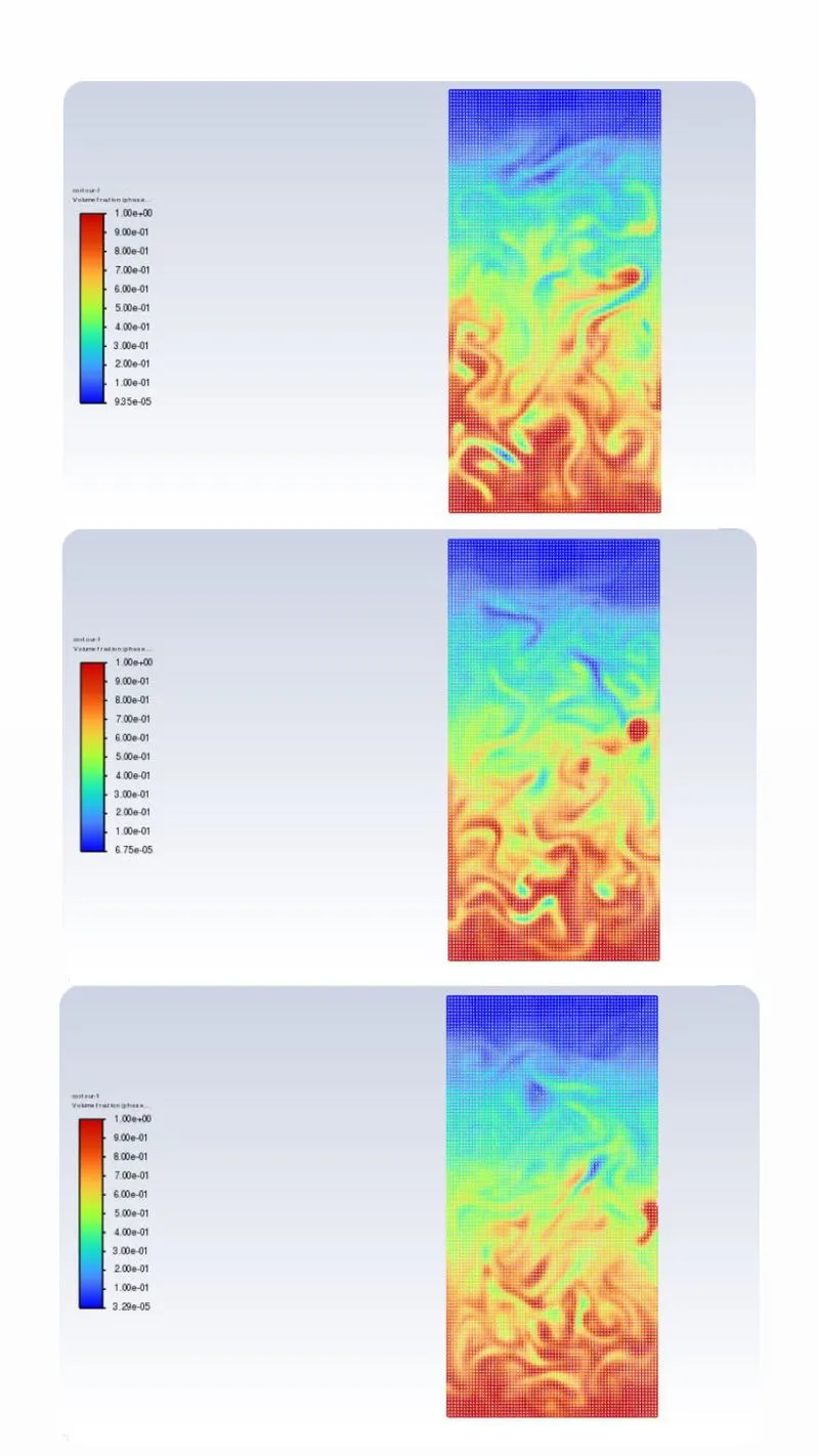
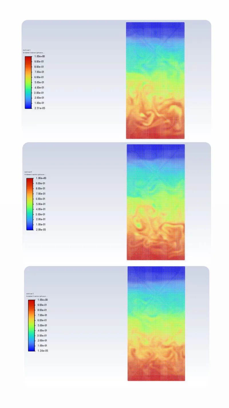
Animation
https://drive.google.com/file/d/1VqU1a_5_MVUayzz_0D0kt-t8qqBZNe1d/view?usp=share_link
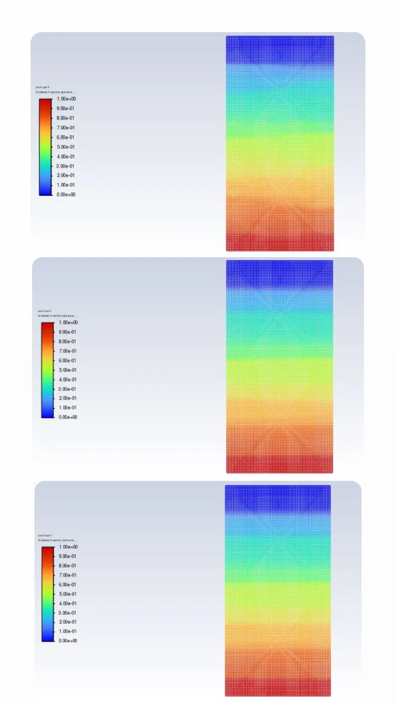
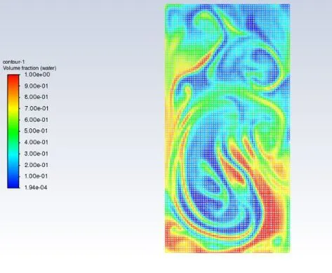
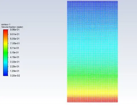
Case 3: simulation with water and user-defined material(density = 400 kg/m3, viscosity = 0.001 kg/m-s) for refined mesh.
Scaled Residuals
The contour of the volume fraction
Animation
https://drive.google.com/file/d/1j1B7PMDxGecT5seLpXbcZ7GgU2TYqo_1/view?usp=share_link
Why a steady-state approach might not be suitable for these types of simulations?
The steady-state analysis is used when we are more concerned with the end result. But for Rayleigh Taylor instability we are more interested in observing the real-time changes of the interface and the fluid region. Real-time observation is possible in Transient State analysis.
The difference between the steady and transient is that you can't see the small-time variation of instability. The steady-state simulation is performed if we are concerned more about the final state results or the equilibrium state. In RT-Instability CFD models, we are more concerned to learn about the transition of the irregularities that starts developing when we pour highly dense fluid upon low dense fluid under gravity effect so, by using a transient solver along with a refined mesh of the model, we can compute the smooth transition of irregularities that takes place at the interface of the fluids. The final state results for both the steady-state and transient-state will be the same.
This simulation cannot be run under steady-state conditions because it changes from time to time iterations so we cant achieve this simulation through this condition.
Atwood number:
It is a dimensionless number in fluid dynamics used in the study of hydrodynamic instabilities in density-stratified flows. It is a dimensionless density ratio defined as
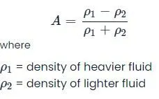
Find out the Atwood number for this case and explain how the variation in the Atwood number affects the behavior of the instability.
The Atwood number for the above case is
A = (998.2-1.225)/(998.2+1.225)
A = 0.9975
When the Atwood number is so high more instability takes place in the fluid and measuring the spikes of the instability is very difficult.
When the Atwood number is low the more stable the fluid mixture and measuring the spikes of the instability can be done to some extent because it expresses linearity to some extent.
How can we use the Atwood number to validate our simulation result?
Significance:
Penetration distance of the heavier fluid into the lighter fluid is given by the formula Agt^2 where g is the acceleration due to gravity and t is the time.
For A close to 0, RT instability flows take the form of symmetric fingers of fluid.
For A close to 1, the much lighter fluid below the heavier fluid takes the form of larger bubble-like plumes.
For this case
A = (998.2-1.225)/(998.2+1.225)
A = 0.9975
we see that the lighter fluid (air) rises up and bubble-like plumes take place. The Atwood number calculated for our result is close to 1. The Atwood number close to 1 signifies the same phenomenon. And hence validates our result.
Conclusion:
Rayleigh Taylor's instability was observed at the interface of the fluids with different densities under the influence of gravity. Since the simulation involves capturing instabilities that are changing in an unpredictable manner as a function of time, the transient approach is preferred over the steady-state approach.
The lower-density fluid pushes the higher-density fluid above it. The heavier fluid which is water, in this case, comes to the bottom and replaces the air from the bottom.
The formation of air bubbles takes place which moves upward.
The mesh refinement leads to a better simulation of the Rayleigh Taylor instability. All the instability and the irregularities that take place at the interface are better visualized as we refined the mesh.
In all cases, the lower-dense fluid pierces into the high-density fluid as it seems to be the propagation of a shock wave.
In case 1 at the interface, we can see that some disturbances are formed as time passed the large disturbance is formed by its forces into the highly dense fluid like a shock wave.
In case 2 at the interface, we can see the disturbances which are more than in case 1 pushing through the highly dense fluid mushroom-like structure is formed and formation of bubbles can be seen around the mushroom structure.
In case 3 at the interface disturbances are observed in more detail in the form of many bubbles and the formation of vortices can be clearly seen.
After performing the 3 case setups with respective base grid sizes the cases 2 & 3 we can see that there were only minor changes in the post-processing results showing us that the case had converged. The finer the mesh the greater the possibility of accurate flow prediction. Here Case 3 has the finest mesh of all. So can we take data from case 3 since it will have an accurate simulation result.
From the above cases, we observe that finer mesh captures the instability better than the coarse mesh, but it takes more time for the heavier fluid to settle down. As computational time is long but produces results with better accuracy.
By comparing all the cases I came to the conclusion that as we go on decreasing the mesh size the mixing of both fluids will get more smooth and more realistic to the physical case, the finer the mesh greater the smoothness in mixing has been achieved.
The steady-state analysis can not be used in this case because in the steady state we focus only on End results. But here in this scenario, we have to carry out results and record them for each time step so that we can observe the intermediate behavior of fluids, That's Why transient analysis is a must in this case to capture the intermediate relations and behavior of mixing fluid.
The Atwood number validates the CFD simulation as it is observed. In the case of water and air mixing, bubble formation takes place, whereas in the other case no bubble takes place.