Week 5 - Rayleigh Taylor Instability

Rayleigh Taylor Instability

Aim

studying the Rayleigh Taylor Instability on the two different density fluids

Introduction

Rayleigh-Taylor (RT) instability takes place when a lighter fluid supports a heavy fluid, then any perturbation of the interface grows and leads to spikes of the heavier fluid penetrating into the lighter one and the interface becomes unstable.

Solving & Modelling approach

1. Perform the Rayleigh Taylor instability simulation for 2 different mesh sizes with the base mesh being 0.5 mm. Compare the results by showing the animations( Attach them from your google drive). Observe the differences in the animation and explain the effect of mesh size on simulation. Also, explain why a steady-state approach might not be suitable for these types of simulation.[ Choose Air and Water for this simulation]
2. Run one more simulation with water and user-defined material(density = 400 kg/m³, viscosity = 0.001 kg/m-s) for refined mesh

Pre-processing and solver setting

Geometry

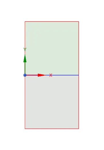
Fluid flow (fluent)--> create the geometry in Space Claim with the Dimensions of 20mmx20mm both surfaces and seprated with different components names as water and air

The physics must share between the two surfaces for the apply share topology on the interface area (indicated as blue line)

Meshing

Case 1

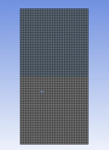
Base mesh size of 0.5 mm

Setup

Solver Type	Pressure-Based
Velocity Formulation	Absolute
Time	Un-Steady
Models	Viscous model: laminar Multiphase: Volume of fluid : Implicit formulation : 2 phases
Material	Fluid type: Air : water liquid Solid-type: Aluminium
Cell zones	Fluid type: Air : water
Boundaries	Standard
Reference values	Standard
Initialization	Standard Patch: Water-surface (1 value of volume fraction of water) : Air-surface(0 value of volume fraction of water)

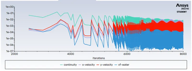
Residuals

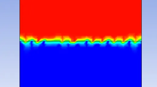
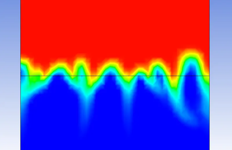
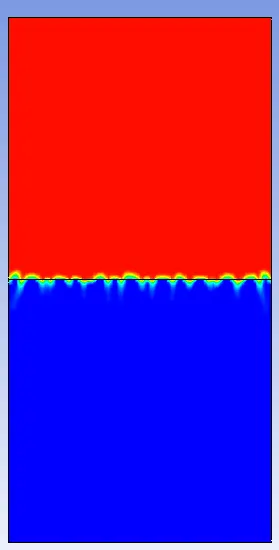
instability in interface of the two fluids

stage 1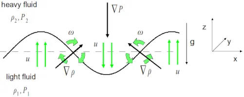

stage-2

stage 3

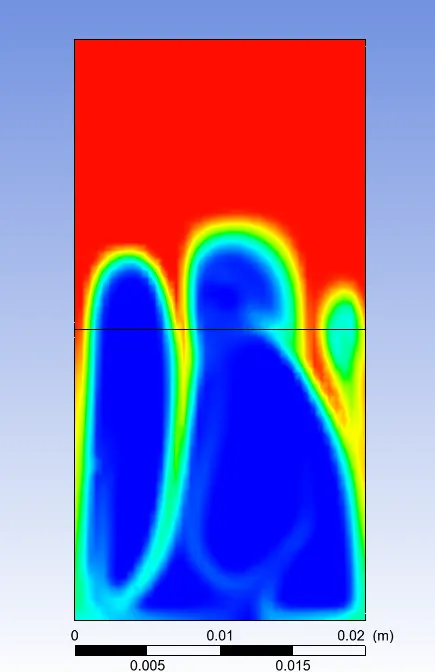
satge-4

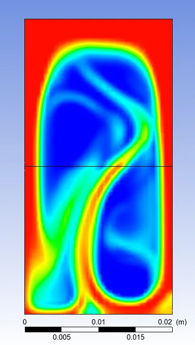
stage-5

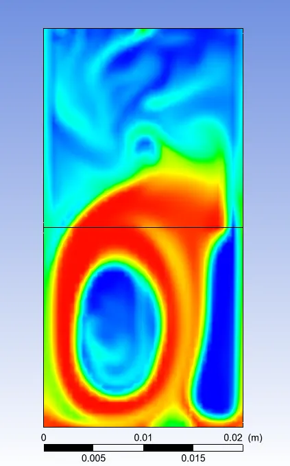
stage- 6

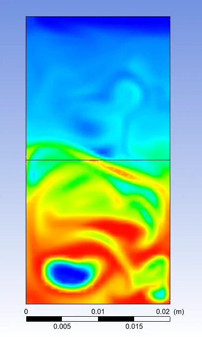
stage-7

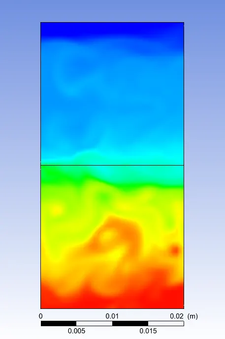
stage -8

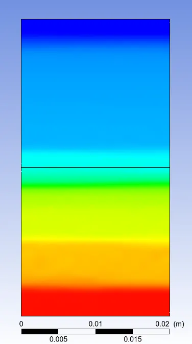
Case - 2

Case -2

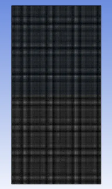
target length = 0.2mm

Setup

Solver Type	Pressure-Based
Velocity Formulation	Absolute
Time	Un-Steady
Models	Viscous model: laminar Multiphase: Volume of fluid : Implicit formulation : 2 phases
Material	Fluid type: User-defined-fluid(Density =400 kg/m3, viscosity = 0.001 kg/m-s) : water liquid Solid-type: Aluminium
Cell zones	Fluid type: Air : water
Boundaries	Standard
Reference values	Standard
Initialization	Standard Patch: Water-surface (1 value of volume fraction of water) : Air-surface(0 value of volume fraction of water)

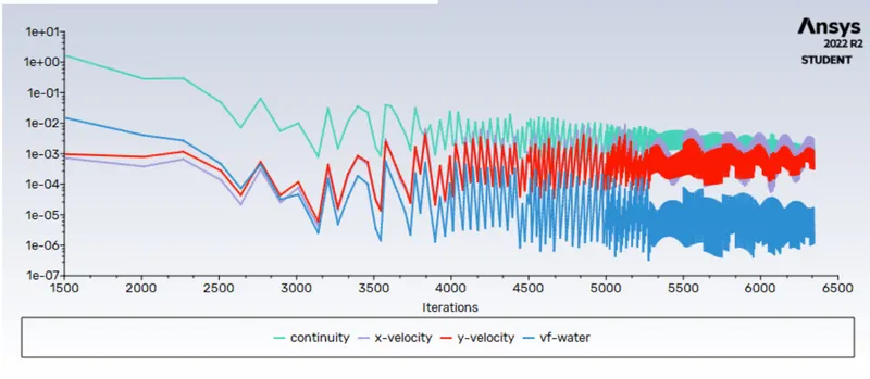
Residual

stage -1

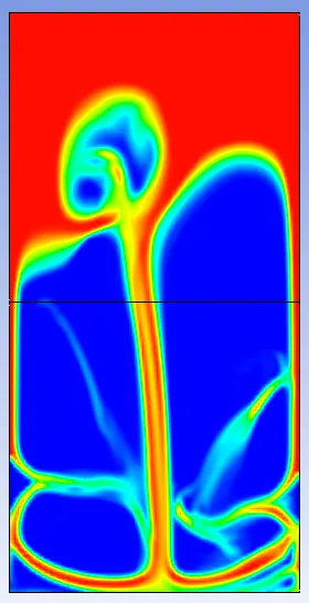
stage -2

stage -3

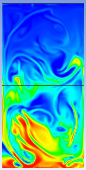
stage-4

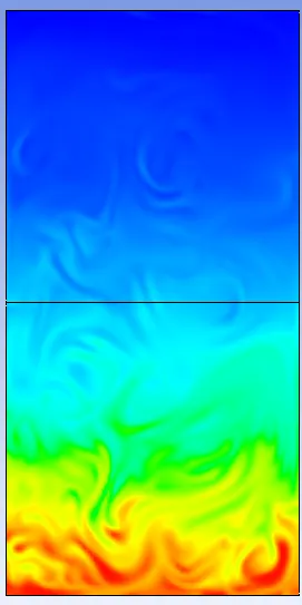
stage-5

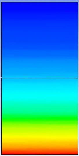
Atwood number

The Atwood number is a dimensionless number in fluid dynamics used in the study of hydrodynamic instabilities in density-stratified flows. The Atwood number equals the ratio of the difference in mass densities to their sum.

A = ρ1 - ρ2 / ρ1 + ρ2

case -1

density of air = 1.225 kg/m³

density of water = 997 kg/m³

A = (1.225 - 997) / (1.225 + 997)

A = 0.997

case -2

density of air = 1.225 kg/m³

density of water = 400 kg/m³

A = (1.225 - 400) / (1.225 + 400)

A = 0.994

CONCLUSION:

• From the above cases, we observe that finer mesh captures the instability better than the coarse mesh, but it takes more time for the heavier fluid to settle down. As computational time is long but produces results with better accuracy.
• Since the simulation involves capturing instabilities that are changing in an unpredictable manner as a function of time, the transient approach is preferred over the steady-state approach.
• The Atwood no validates the CFD simulation as it is observed. In the case of water and air mixing, bubble formation takes place, whereas in the other case no bubble takes place.