Week 5 - Rayleigh Taylor Instability
Aim :- Perform the Rayleigh Taylor instability simulation for 2 different mesh sizes with the base mesh being 0.5 mm. With addition a new setup with a user material property has been simulated to understand the instability phenomenon. Atwood number computation is also carried out to predict the corresponding CFD solutions.
Objectives :-
- What are some practical CFD models that have been based on the mathematical analysis of Rayleigh Taylor waves? Explain how these mathematical models have been adapted for CFD calculations.
- Perform the Rayleigh Taylor instability simulation for 2 different mesh sizes with the base mesh being 0.5 mm. Compare the results by showing the animations( Attach them from your google drive or convert in into gif file then attach it). Observe the differences in the animation and explain the effect of mesh size on simulation. Also, explain why a steady-state approach might not be suitable for these types of simulation.[ Choose Air and Water for this simulation]
- Run one more simulation with water and user-defined material(density = 400 kg/m3, viscosity = 0.001 kg/m-s) for refined mesh.
- Define the Atwood Number. Find out the Atwood number for both the cases and explain how the variation in Atwood number in the above two cases affects the behavior of the instability.
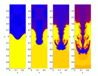
Rayleigh Taylor Instability :- The Rayleigh Taylor instability is an instability of an interface between two fluids of different densities which occurs when the lighter fluid is pushing the heavier fluid in a gravitational field. Examples include the behavior of water suspended above oil in the gravity of earth.
The study focuses on the transient state simulation of Rayleigh Taylor waves and subsequent turbulent mixing in the two phases incorporated in the model.
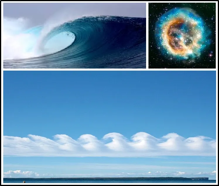
- Kelvin–Helmholtz instability: The Kelvin–Helmholtz instability is a fluid instability that occurs when there is a velocity difference across the interface between two fluids. Kelvin-Helmholtz instabilities are visible in the atmospheres of planets and moons, such as in cloud formation on Earth
- Richtmyer–Meshkov instability: The Richtmyer–Meshkov instability (RMI) occurs when two fluids of different density are impulsively accelerated.
- Plateau–Rayleigh instability: The Plateau–Rayleigh instability, often just called the Rayleigh instability, explains why and how a falling stream of fluid breaks up into smaller packets with the same volume but less surface area. Example-
Water dripping from a faucet/tap
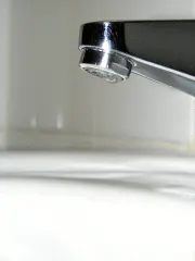 Water dropping from a tap
A special case of this is the formation of small droplets when water is dripping from a faucet/tap. When a segment of water begins to separate from the faucet, a neck is formed and then stretched. If the diameter of the faucet is big enough, the neck doesn't get sucked back in, and it undergoes a Plateau–Rayleigh instability and collapses into a small droplet.

Modelling and problem solving approach:
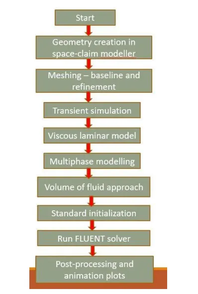
Creation of the Geommetry in spaceclaim :
- Ansys space claim design domain opens up.
- Select a plane to create the domain of air. Select the rectangular tool. Draw a rectangle of 20x20mm.
- Select the pull tool to convert to surface domain. Rename the component as air.
- Now for creating the second component which is water, move to a new component.
- Now to create the water domain, we select the same plane over which we drew the air component. Select the rectangular tool and draw the profile above the air surface.
- Now for checking the topological sharing. Enable the share topology to share the information between this two surface .
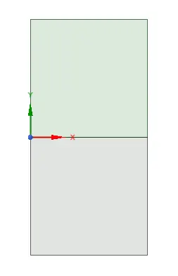
After enable the share topology-
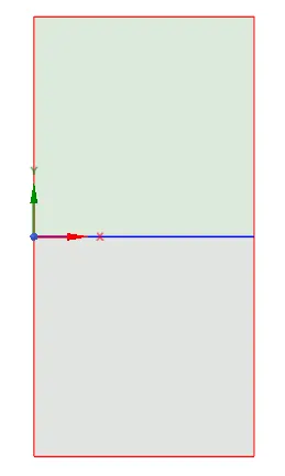
This is our final geometry . Now we can go ahead with meshing the geometry .
Meshing :
- Open the meshing console.
- Click on the mesh and select generate mesh option.
- Now a basic mesh pattern will be created.
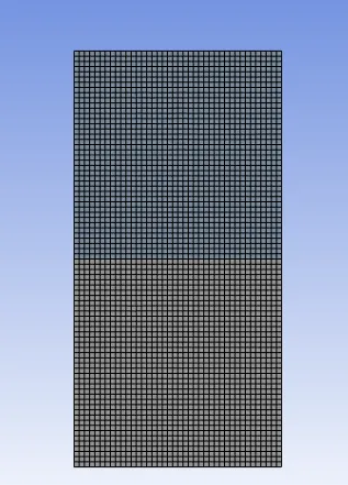
- Now we will run a baseline mesh having size of 0.5mm. We go to mesh size and put the desired value>> click on generate mesh tab.
- Now on the next step we will refine the mesh size by 0.3mm and 0.1mm respectively.
Pre processing set up :
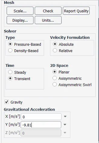
- We will be performing a transient simulation with gravity force acting in the negative y direction. Thats why gravity is -9.81 m/s^2.
And we have choosen Laminar flow as viscous model and will run a multiphase simulation .
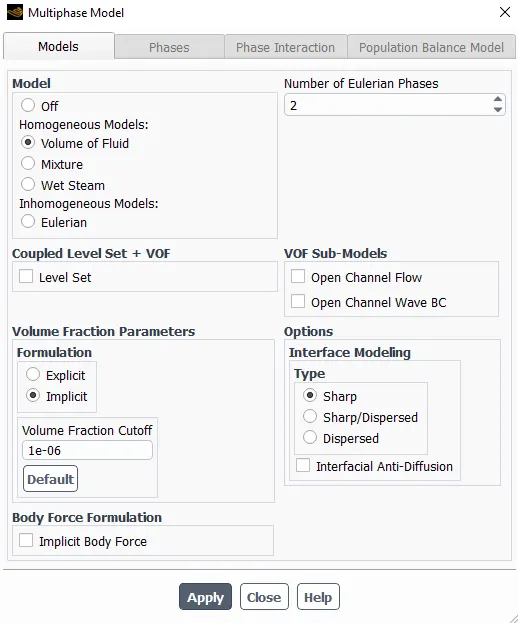
Select the Implicit option as we are not going for courrant number .
Now open the Phases and select the air as primary and water as secondary phase .
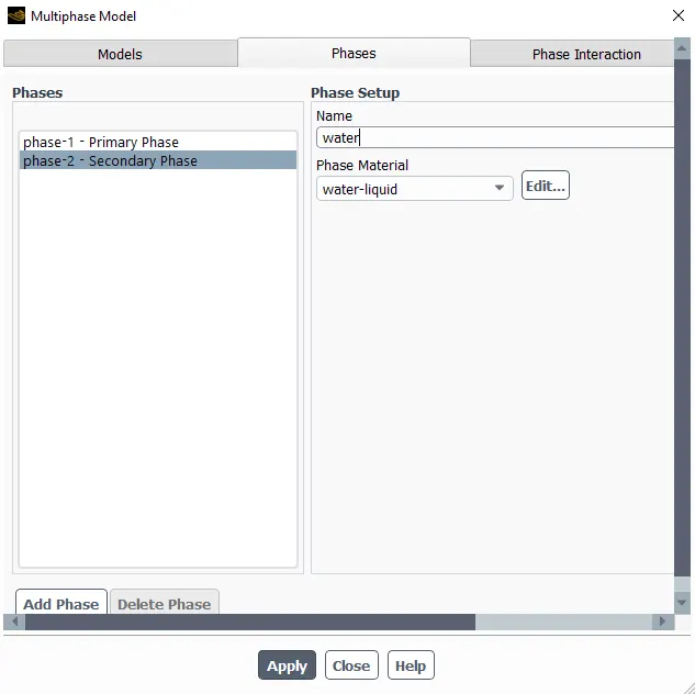
Now to define the material. Go to material section. Select water from fluent database , copy and close.
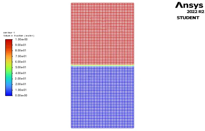
Then initializing the problem. Here we will looking for the standard initialization . After creating the patch , contour for water volume fraction has been created .
Now click on auto save to see the animation in post processing and also create solution animation to see the animation in set up itself.
Set the Number of Time Steps and Time Step Size and hit calculate to run the simulation .
Case 1 with Baseline mesh setup :
Meshing (Size = 0.5 mm)
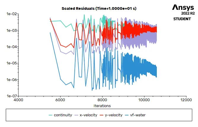
Iteration to converge
Contour before simulation
Water volume fraction contour after simulation
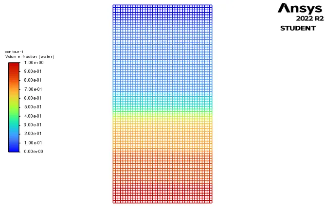
Animation (google drive link)
https://drive.google.com/file/d/1Y174501dGxLzzlfm4GzUG6TkzNCJStbG/view?usp=sharing
Case 2 with Refined mesh setup :
Meshing (Size = 0.3 mm)
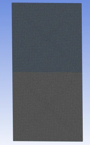
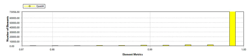
Quality criteria
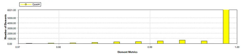
Iteration to converge
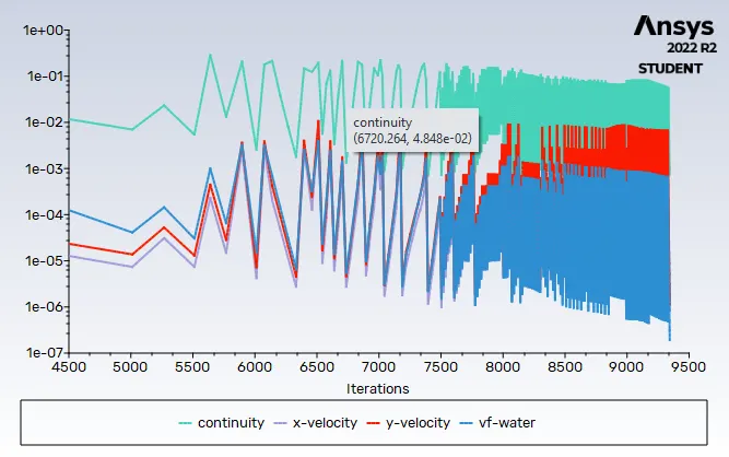
Water volume fraction contour after simulation
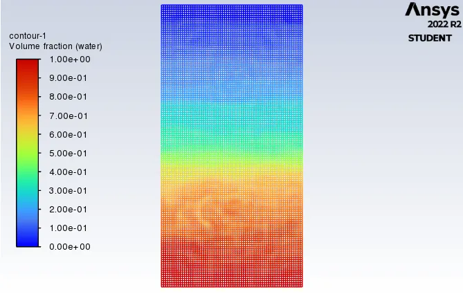
Animation (Google drive link)
https://drive.google.com/file/d/1PERBb6KndiLnZJxyfPAPhHweMyvezU3D/view?usp=sharing
Case 3 with Refined mesh setup :
Meshing (Size = 0.1 mm)
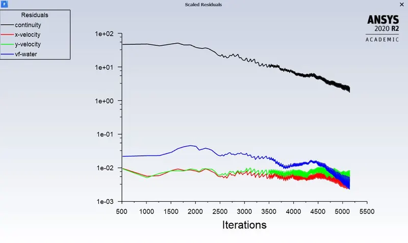
Iteration to converge
Water volume fraction contour after simulation
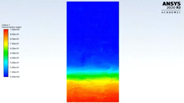
Animation (Google drive link)
https://drive.google.com/file/d/1Hcu-_QjtoK047a9hDUrkhbj9caa5715r/view?usp=sharing
Case 4 with Refined mesh setup (User material):
FLUID:
USER MATERIAL DENSITY: 400
WATER DENSITY:1000
Meshing (Size = 0.1 mm)
Mesh Quality criteria
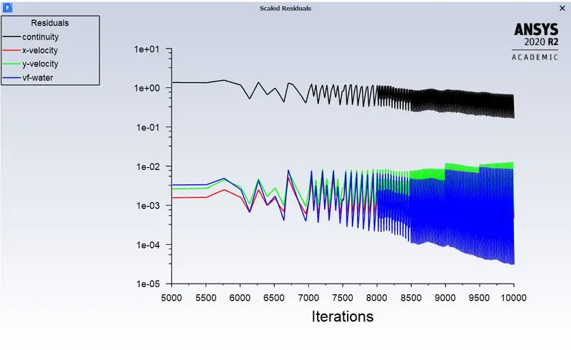
Iteration to converge
Water volume fraction contour after simulation
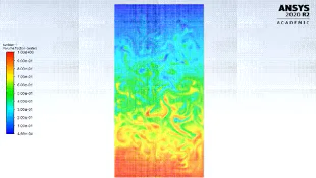
Animation (Google drive link)
https://drive.google.com/file/d/1C15PnZPvv-MsdkFEz1xJUfv-LeM4PvaH/view?usp=sharing
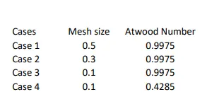
Atwood Number :- The Atwood number (A) is a dimensionless number in fluid dynamics used in the study of hydrodynamic instabilities in density stratified flows. The difference in the fluid densities divided by their sum is defined as the Atwood number, A . It is a dimensionless density ratio defined as
`A = (rho1-rho2)/(rho1+rho2)`
where
- `rho1`= density of heavier fluid
- `rho2`= density of lighter fluid
Atwood number for Case 1
A = `(1000-1.22)/(1000+1.22)`
= 0.9975
where 1000 is the density of water
1.22 is the density of air
Atwood number for Case 2 , 3 and 4 is the working property fluid and water are same for both of this cases.
Atwood number for Case 4
A = `(1000-400)/(1000+400)`
= 0.4285
where 400 is the density of the user material for Case 4
Observation/Conclusion:
1. With increasing the mesh size or number of total elements , the more correct the observation of bubble formation can be captured.
2.Incorrect time steps or large courant no can lead to floating point errors. So required relaxation factors should be given accordingly.
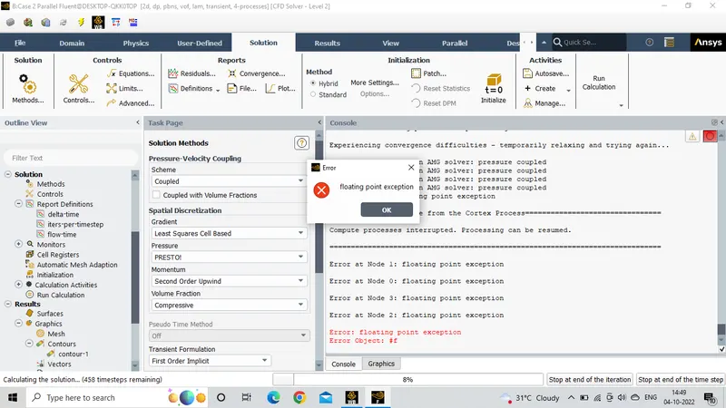
To deal with this error we need to use small Time Step Size .
3.With increase in mesh refinement, the computational time increases.
4.The Atwood no validates the CFD simulation as it is observed. In case of water and air mixing, bubble formation takes place, whereas for the other case no bubble takes place.
References :-
https://skill-lync.com/knowledgebase/how-to-overcome-floating-point-exception-error