Week 5 - Rayleigh Taylor Instability

RAYLEIGH TAYLOR INSTABILITY

Introduction:

Rayleigh Taylor Waves

Rayleigh-Taylor waves describe an instability of an interface between two fluids of different densities which occurs when the lighter fluid is pushing the heavier fluid. Beginning from a state of hydrostatic equilibrium in a constant gravitational field, RT instability at the interface will launch a shock wave into the upper fluid. The rising bubbles of light fluid act like pistons, compressing the heavy fluid ahead of the fronts and generating shocklets. These shocklets coalesce in a multidimensional fashion into a strong normal shock, which strengthens as it propagates upwards.

CFD models based on Rayleigh Taylor Instability

Richtmyer-Mishkov instability: This instability occurs when two fluids of different densities are impulsively accelerated. This happens due to shockwaves normally. small perturbations which grow linearly with time starts the instability. Then the non-linear regime with bubbles of lighter fluid penetrates the heavier fluid. Spikes can also be seen while heavier fluid penetrating a lighter fluid. a chaotic regime with mixing of fluids is reached. This is an impulsive-accelerated limit of RT instability.

Plateau-Rayleigh instability: This is just another case of RT instability, which explains why and how a falling stream of fluid breaks up into smaller packets with the same volume but less surface area. This theory widely explains the occurrence of fluid thread breakup. It is employed in ink jet technology where a jet of liquid ink is perturbed into a steady steam of droplets. This theory is driven mainly by the surface tension of the liquid phase to minimize their surface area.

Kelvin-Helmholtz instability: This fluid instability occurs when there is a velocity shear in a single continuous fluid or a velocity difference across the interface between two fluids. It is observed visible in the atmospheres of planets and moons such as cloud formations on Earth and red spot on Jupiter and the atmospheres of the sun and other stars

Discrete Boltzmann model: It is suitable for investigating the hydrodynamic and thermodynamic non-equilibrium effects in phase separation processes. It is used to estimate the deviation amplitude from the thermodynamic equilibrium. The cases of premixed, non-premixed and partially premixed non-equilibrium reactive flows are studied across subsonic and supersonic flows.

Smoothed Particles Hydrodynamics: It is computational method used for simulating the mechanics of continuum media such ad solid mechanics and fluid flows. It was initially developed for astrophysical problems. It has been used in many fields of research including ballistics, volcanology and oceanography. It is a meshfree lagrangian method and the resolution of the method can be easily adjusted with respect to variables such as density.

Single Fluid Model: It is the analysis of two-phase flows in a mixture model. The individual fluid phases are assumed to behave as a flowing mixture described in terms of the mixture properties. It is a five-equation model consisting of the mass, momentum and energy equations for a vapour/liquid mixture and two equations describing the formation and growth of the liquid phase.

Two Fluid Model: In this model, the separate sets of governing equations for vapour and liquid phases have been used. Here also, the interaction between the droplets, the heat exchange between the liquid phase and the solid boundary are not modeled. Also the velocity slip between the vapour and the liquid phase is taken into considerations.

Turbulence Model: Turbulence model predicts the average mixing behaviour inflows that are on average 1D or 2D. Experimental results are used to build the turbulence model. The equations governing turbulent flows can only be solved directly for simple cases of flow. In Computational dynamics, the statistical evolution of turbulent flows are based on the simplified constitute equations.

Atwood Number

It is a dimensionless density ratio, used in fluid dynamics to study the hydrodynamic instabilities in a density stratified flow, typically used in Rayleigh Taylor instability and Richtmyer-Mishkov instability.

Atwood number is given by the relation, `(rho1-rho2)/(rho1+rho2)`, where `rho1`is the density of the heavier fluid and `rho2`is the density of the lighter fluid.

Theoretically, the penetration of the heavier fluid bubbles into the lighter fluid is a function of an accelerated time relation, given by `Ag t^2`, where g is the acceleration due to gravity, t is the time, A is the Atwood number

Procedure:

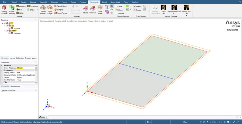
Step 1: Setting up the geometry

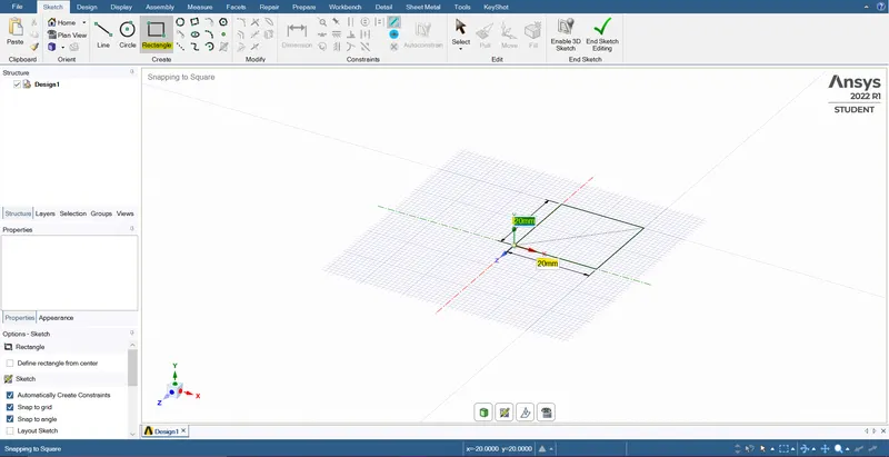
Sketch a square using the rectangle command of size 20*20 mm

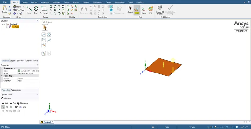
Use Pull command to convert the square to a surface.

Sketch another square for the water surface, and move to a new component.

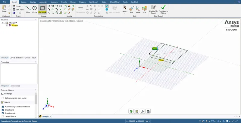
Use the pull command again to make it a surface and rename as the water surface.

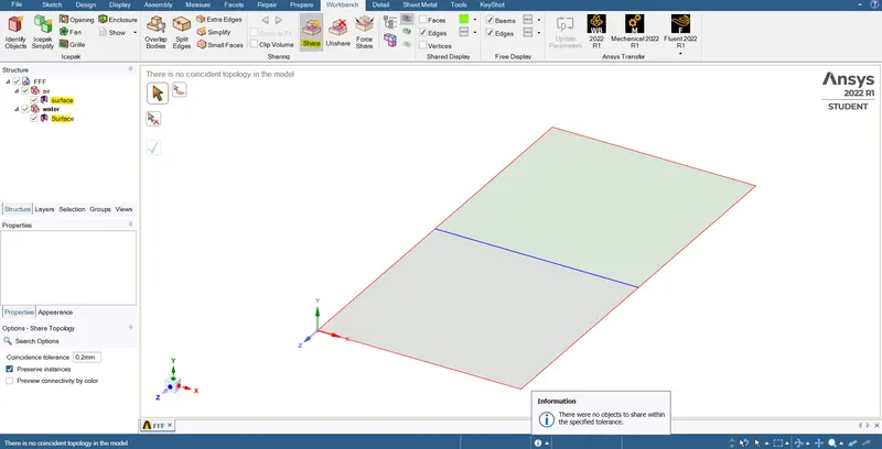
Move both the surfaces to a new component under the same design and enable topology sharing between the two surfaces.

Step 2: Meshing

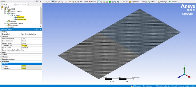
Element sizes between 0.5mm to 0.1mm is given to generate a computable mesh grid.

Step 3: Setup

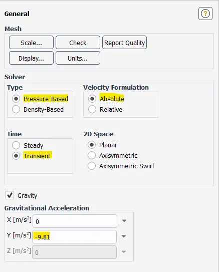
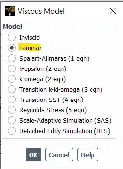
The general setup is set with a pressure based solver in a laminar - transient model and the gravity is given as -9.81m/s in the Y direction.

The fluid material water is loaded from the fluent database and is checked for properties.

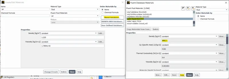
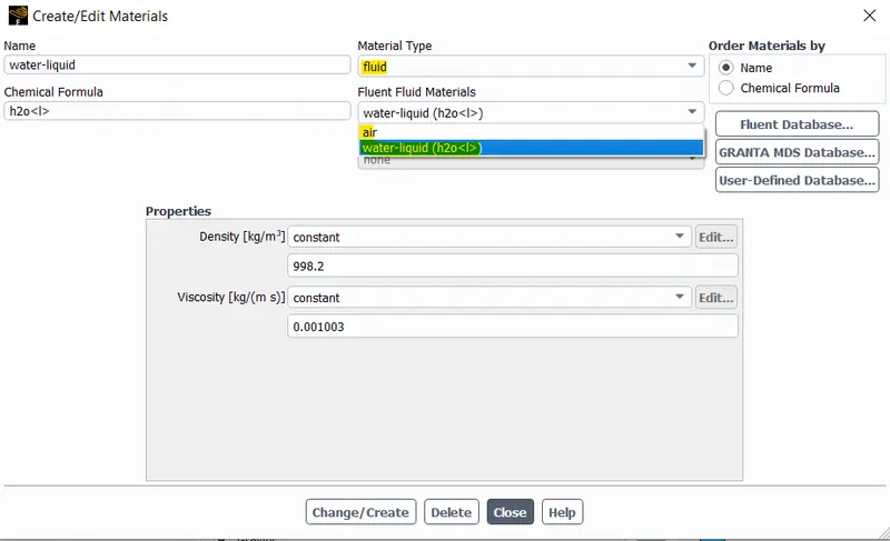
Both the materials of air and water are loaded in materials database.

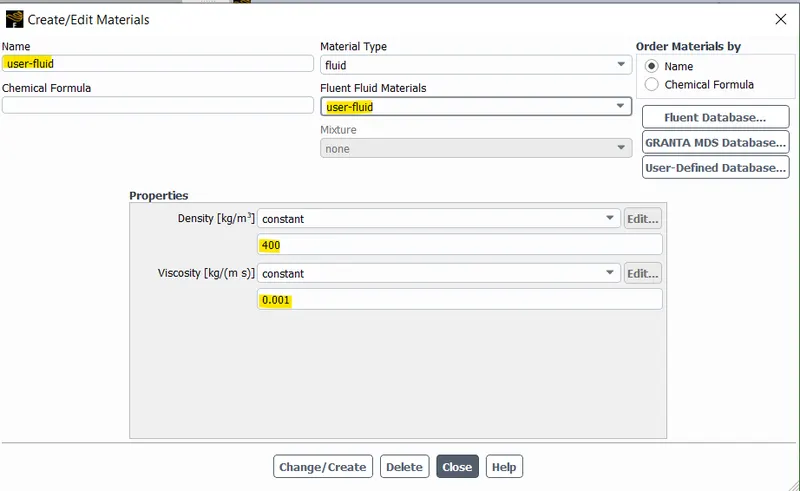
A user defined fluid with density 400kg/m3 and viscosity 0.001 kg/m-s is made by copying the properties of water or air.

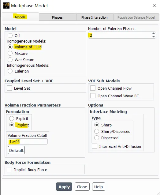
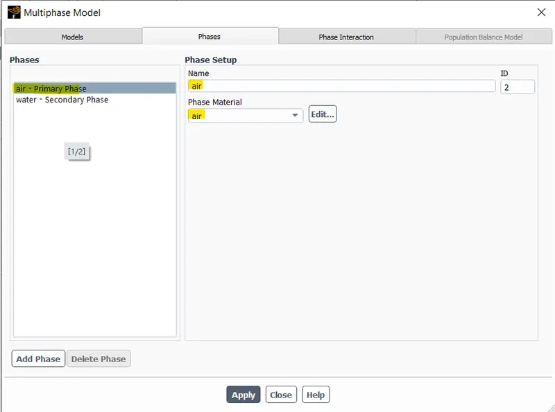
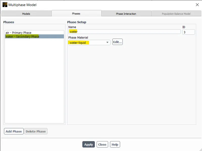
The multiphase model is constructed with volume of fluid method, and the primary phase is set to air, the secondary phase is set to water.

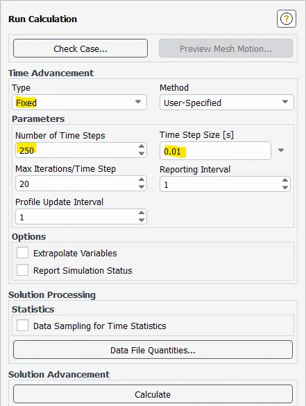
The time step size is adjusted between 0.025 to 0.005 while the number of time steps is kept at 250, and standard initialization is done for the solution.

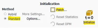
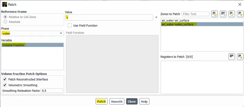
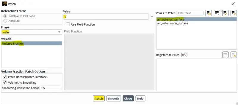
Patching is done after the initialization process for water phase and the volume fraction is set to 1 in the water surface and the volume fraction is set to 0 in the air surface.

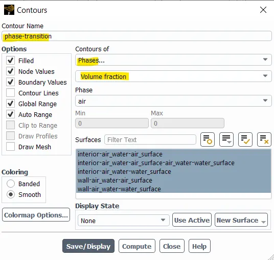
A contour and animation for the phase transition is defined in all the surfaces of the geometry.

Cases:

Baseline case	Refined case	Refined comparative case
Air-Water phases Mesh size: 0.5mm Laminar - Transient model Intrinsic discretization 250 timesteps time step size: 0.02	Air-water phases Mesh size:0.25mm Laminar - Transient model Intrinsic discretization 250 timesteps time step size: 0.01	Water-User defined phase (density = 400 kg/m3, viscosity = 0.001 kg/m-s) Mesh size: 0.25mm Laminar - Transient model Intrinsic discretization 300 timesteps time step size: 0.015

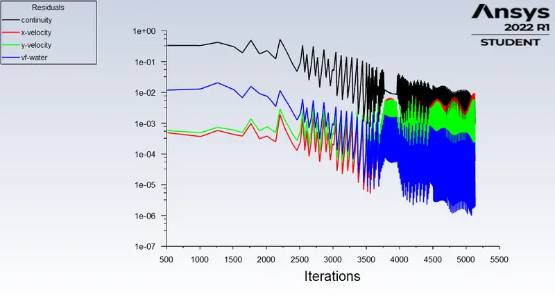
Results:

Baseline case	Refined case	Refined comparative case

Inference:

Baseline case animation	Refined case animation	Refined comparative case animation
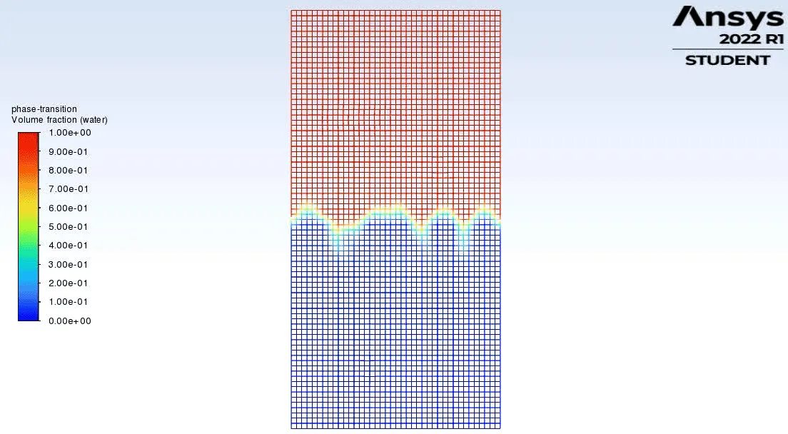
Atwood number = `(998.2-1.225)/(998.2+1.225)` = 0.9975	Atwood number = `(998.2-1.225)/(998.2+1.225)`= 0.9975	Atwood number = `(998.2-400)/(998.2+400)` = 0.4277

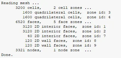
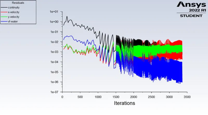
Baseline case: In this case, the mesh size is 0.5m which had only 3200 cells. The time step is maintained at 0.02 as, 0.025 and above resulted in floating point exception. Since the mesh cells are bigger, we could see larger air bubbles pushing their way upward into the water phase. The time step size also indicates that the instability takes only 0.02 second within the mesh and so, the entire instability gets stable around 180 time steps which is nearly 3.6 seconds. The Atwood number of 0.997 explains the faster acceleration of water particles into the air phase in bigger bubbles.

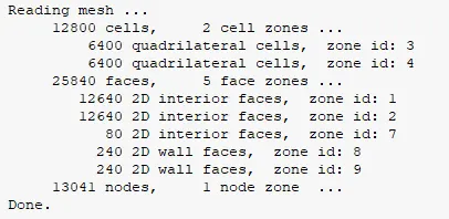
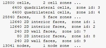
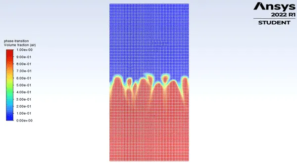
Refined case: In this case, the mesh size is refined to 0.25mm, and the number of cells became 12800. The time step of 0.01 is required as for the smaller mesh size, the time step has to be reduced. It is observed that a time step size above 0.01 to 0.025 makes the instability diverged. The size of the bubbles is smaller compared to the baseline case, as the mesh cell size is smaller. This needs a smaller time step and the entire instability gets stable at 150 timesteps which is 1.5 seconds. The atwood number has the same value of 0.997 and so the acceleration of water bubbles is the same.

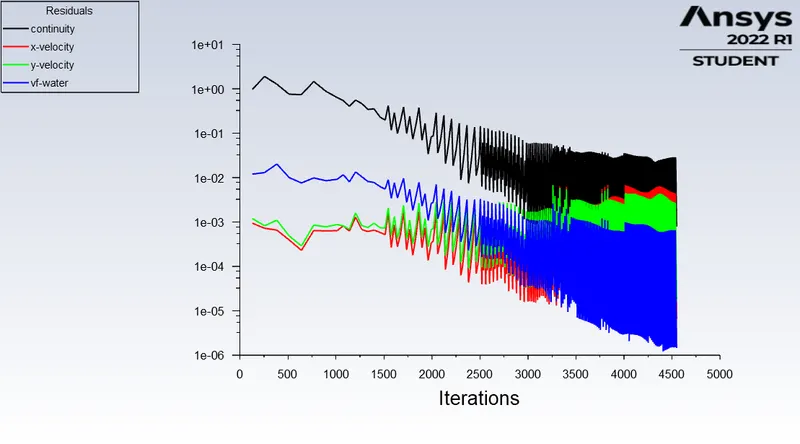
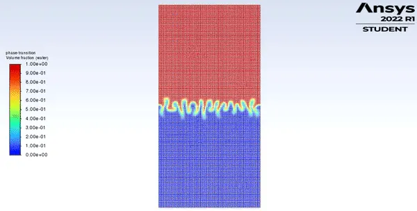
Comparative case: In this case, the mesh size is again 0.25mm with 12800 cells and so the time step required is 0.015 for a convenient simulation. The size of the bubble is smaller when compared to the baseline case, but the acceleration rate is more rapid in accordance with the low atwood number of 0.4277. The entire disturbances seem to settle down at about 200 time steps which is 3 seconds, and is longer than the refined case.

Conclusion:

The Rayleigh taylor instability is studied with different fluids and mesh sizes and the simulation results are plotted which are in accordance with the theoretical atwood number. The atwood number has 3 distinct stages, the linear stability stage, bubble formation and rising, long term evolution duep to bubble merging and mixing. For low atwood number, the linear stage and bubble formation stage are symmetrical to an extent and hence the disturbances are linear for a longer duration. In contrast, for larger atwood number, the linear stability and bubble formation stage is asymmetrical and hence the acceleration rate is rapid, leading to a non-linear stability.