Week 5 - Rayleigh Taylor Instability

AIM:

To study the following

1. To name some practical CFD models that have been based on the mathematical analysis of Rayleigh Taylor waves and to explain how these mathematical models have been adapted for CFD calculations.
2. To perform the Rayleigh Taylor instability simulation for 2 different mesh sizes with the base mesh being 0.5 mm. Compare the results by showing the animations. Observe the differences in the animation and explain the effect of mesh size on simulation. Also, explain why a steady-state approach might not be suitable for these types of simulation.[ Choose Air and Water for this simulation]
3. To run one more simulation with water and user-defined material(density = 400 kg/m³, viscosity = 0.001 kg/m-s) for refined mesh.
4. To define the Atwood Number and to find out the Atwood number for both the cases and to explain how the variation in Atwood number in the above two cases affects the behavior of the instability.

DESCRIPTION:

The Rayleigh Taylor instablility or RT instability is an instability of an interface between two fluids of different densities which occurs when the lighter fluid is pushing the heavier fluid.

Examples include the behavior of water suspended above oil in the gravity of earth, mushroom clouds like those from volcanic eruptions in which expanding core gas is accelerated into denser shell gas, instablities in plasma fusion reactors and inertial confinement fusion.

Water suspended atop oil is an everyday example of Rayleigh-Taylor instability, and it may be modeled by two completely plane-parallel layers of immiscible fluid, the denser fluid on top of the less dense one and both subject to the earth's gravity. The equilibrium here is unstable to any perturbations or disturbances of the interface: if a parcel of heavier fluid is displaced downward with an equal volume of lighter fluid displaced upwards, the potential energy of the configuration is lower than the initial state.Thus the disturbance will grow and lead to a further release of potential energy, as the denser material moves down under the gravitational field, and the less dense material is further displaced upwards.This was the set-up as studied by Rayleigh. When the fluids are accelerated, with the less dense fluid accelerating into the denser fluid.This occurs deep underwater on the surface of an expanding bubble and in a nuclear explosion.

The different types of instability and some practical CFD models that have been based on the mathematical analysis of Rayleigh Taylor waves

1.RITCHMYER-MESHKOV INSTABILITY:

The Ritchmyer-Meshkov instability arises when a shock wave interacts with an interface separating two different fluids. It combines compressible phenomena, such as shock interaction and refraction, with hydrodynamic instability, including non-linear growth and subsequent transition to turbulence, across a wide range of Mach numbers.

2.PLATEAU-RAYLEIGH INSTABILITY:

The Plateau_Rayleigh instability, often just called the Rayleigh instability, explains why and how a falling stream of fluid breaks up into smaller packets with the same volume but less surface area.This fluid instability is exploited in the design of a particular type of inkjet technology whereby a jet of liquid is perturbed into a steady stream of droplets.

3.KEVIN-HELMOHOLTZ INSTABILITY:

Kevin_Helmholtz instability can occur when there is velocity shear in a single continous fluid, or where there is a velocity difference across the interface between two fluids.An example is a wind blowing over water,The instability manifests in waves on the water surface.More generally, clouds, the ocean, saturn's bands and the sun's corona show this instability.

CASE-I: SIMULATION OF 2D GEOMETRY BY RT INSTABILITY FOR TWO FLUIDS WATER AND AIR

Rayleigh Taylor instability problem, here the idea is we have dense fluid on top and light fluid in bottom and this interface is unstable when gravity is present.

Here our objective is to observe two things

1.How the volume of fluid method is done

2.And how this method serves as the important technique that is used to simulate the two face flows

GEOMETRY

First we create a square

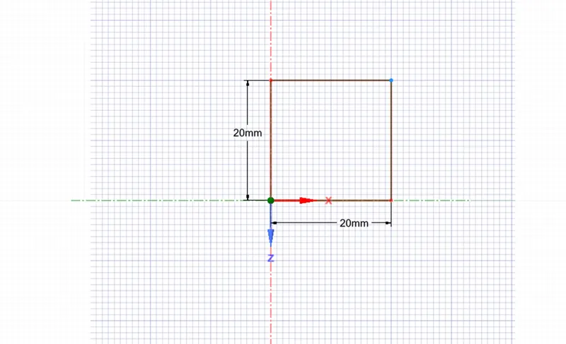
Check for the xy plane during creation

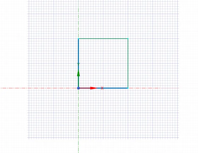
Next we use the pull tool to pull the 2D geometry

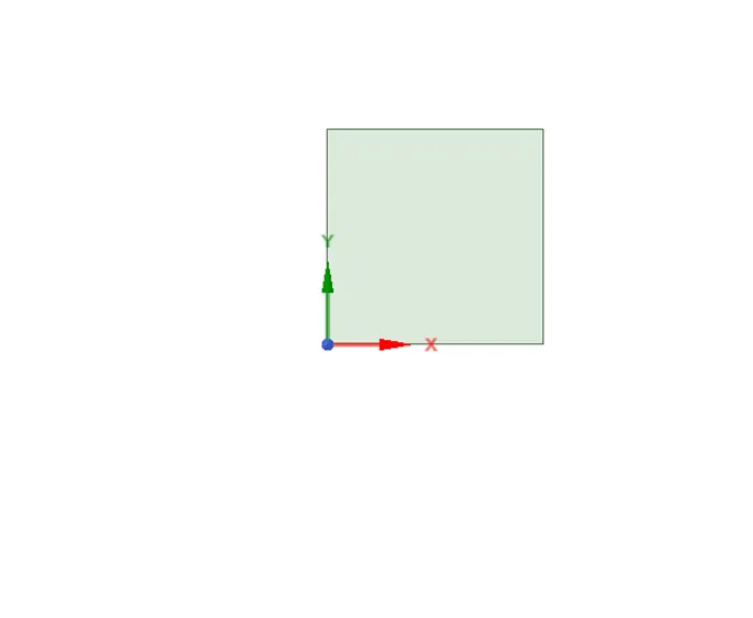
And then moving the surface to the new component by naming it ‘air’

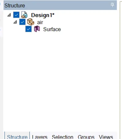
Then selecting the design and creating the new component as ‘water’

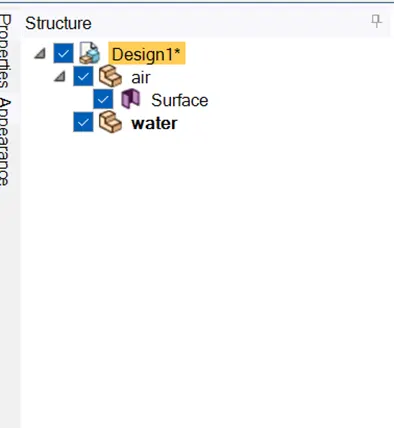
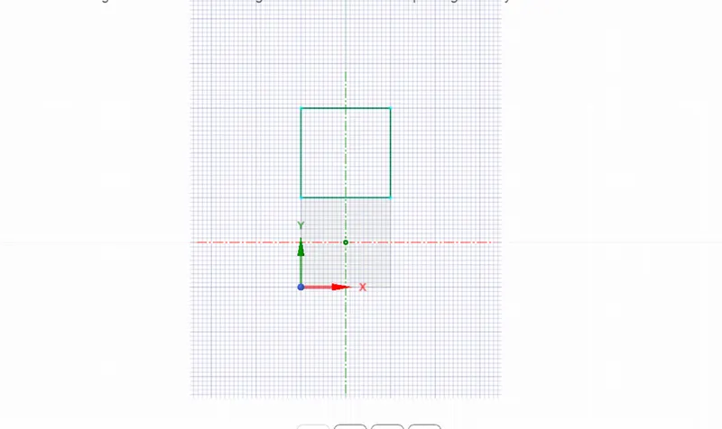
Then selecting water, then sketch mode and selecting the plane and creating another square above it

Then using pull tool to create surface as follows

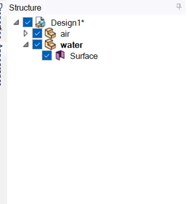
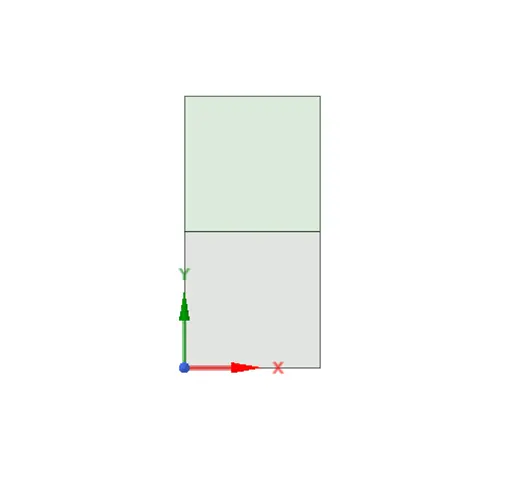
Then using the share tool and select both the surfaces

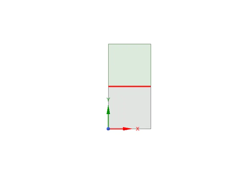
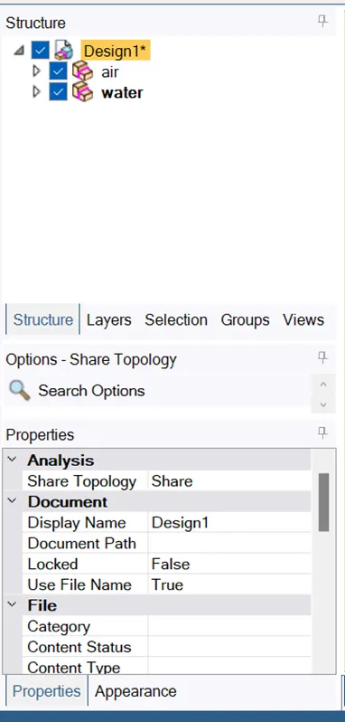
We can see one edge is being shared

We can see also the change in icon and the topology is set to shared

MESHING

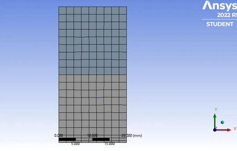
Then generating the default mesh it looks as follows with element size of 2.23mm

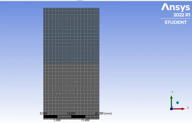
Changing the element size to 0.5mm we get mesh as follows

ANSYS FLUENT

Here we see in graphics the 2D geometry as follows

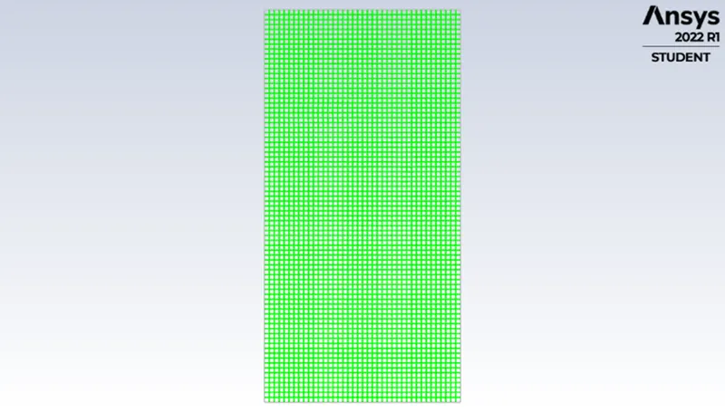
Here we are going for a pressure based solver with transient state because we can see how the interface collapses as a function of time and gravity enabled in negative y-direction we need to check as for geometry

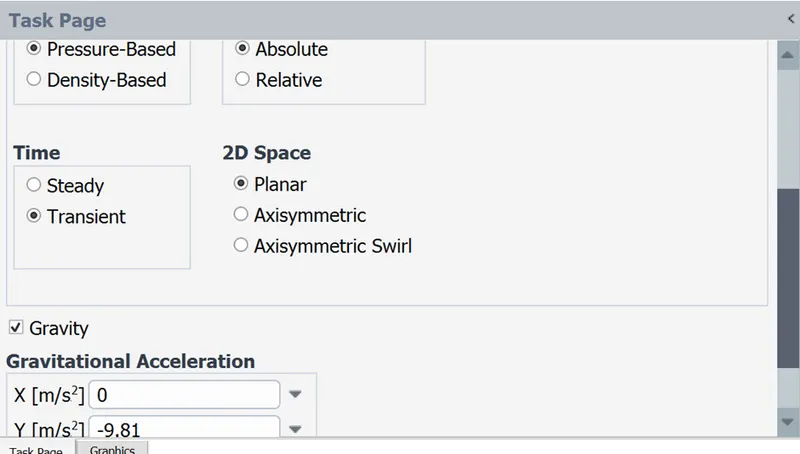
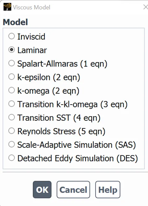
Running for laminar mode

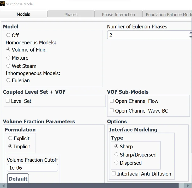
Next we enable the multi-phase model with volume of fluid method, where we have the eulerian phases where 1^st face is air and 2^nd face can be water or vice-versa with implicit formulation

Then for setting up of materials we have air already present, for water we go to fluent databases and copy the water to the materials and we have both the materials

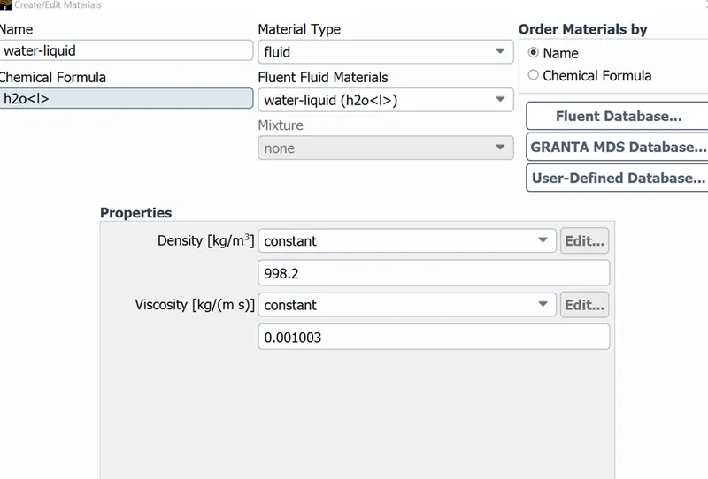
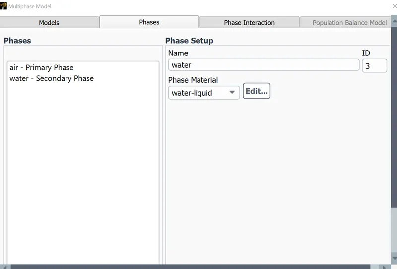
Next changing the phase names to air and water and matching with the fluid type

Next in Domain we check out the zones required

So the top one is water in our case

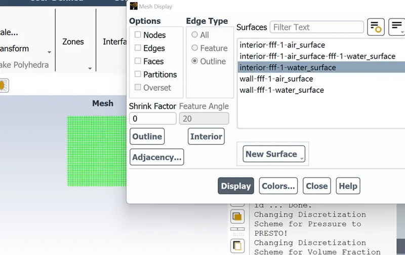
Bottom zone is Air

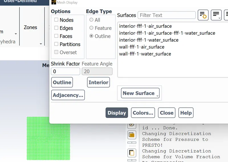
Then after running the standard initialization we see nothing in console but we see some patch option

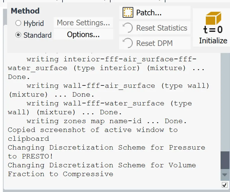
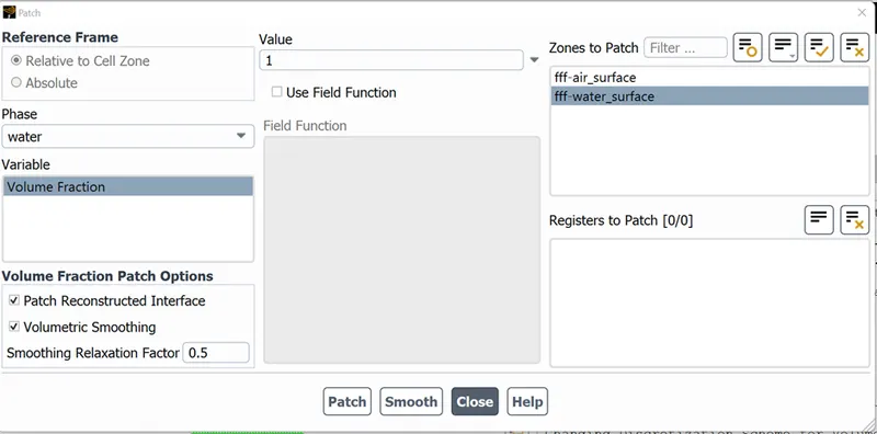
Here in patch we select the water and volume fraction and value as 1 and select the water surface and set the patch

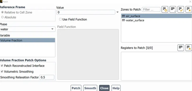
Then for the air surface we give water value as 0 for water and patch it

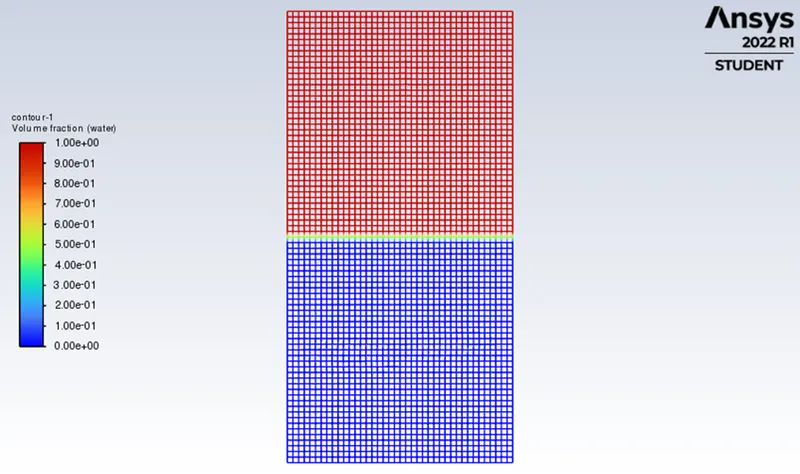
This is because the phases are represented by value alpha; if alpha=1 it represents one phase (water/air) and alpha=0 it represents another phase.This means if alpha=1 is water then if we initialize we mean alpha to be 1 at top and zero at bottom.

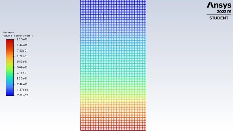
Then we create a contour for phases, with water phase and check for display graphic

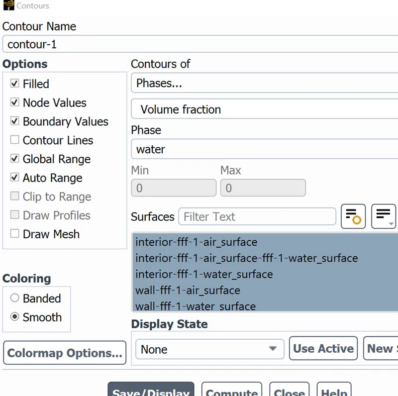
Then creating an animation for contour

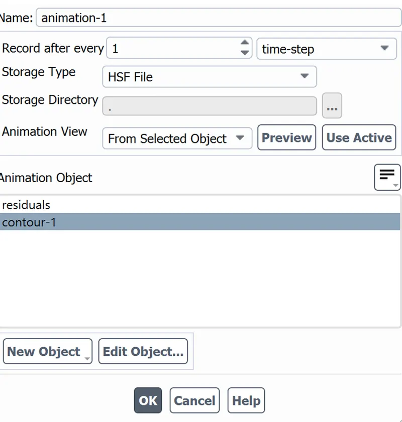
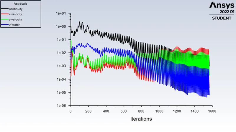
And then running the simulation for 100sec with 0.025 time step

The residual plots is

The phase contour is

https://youtu.be/raoeSlayfI4

CASE-II: SIMULATION OF 2D GEOMETRY WITH FINE MESH OF ELEMENTAL SIZE OF 0.2MM BY RT INSTABILITY FOR TWO FLUIDS WATER AND AIR

Running this case with 0.2mm elemental size mesh, we get as follows

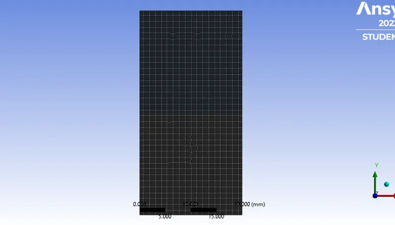
Running the simulation for 1000 timesteps with 0.005 step size

The residual plot is

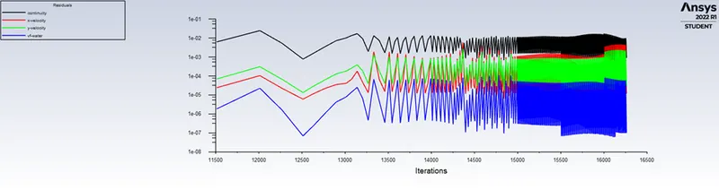
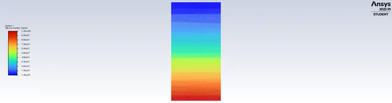
The phase contours is

https://youtu.be/3VYEz7HgOzA

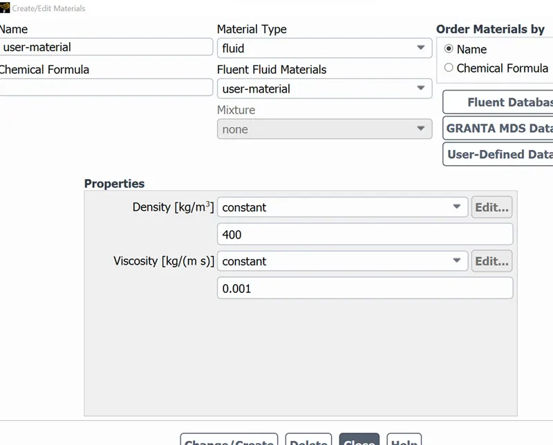
CASE-III: SIMULATION OF 2D GEOMETRY WITH FINE MESH OF ELEMENTAL SIZE OF 0.2MM BY RT INSTABILITY FOR THREE FLUIDS WATER, AIR AND USER MATERIAL (density 400 kg/m3 and viscosity 0.001)

Running the simulation for 500 time steps with step size of 0.005

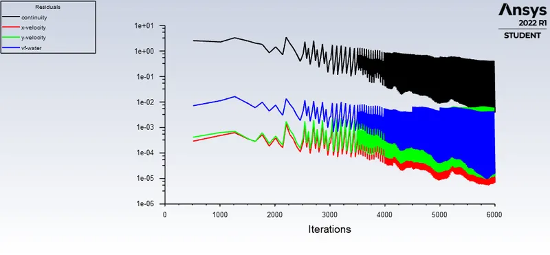
The residual plots are

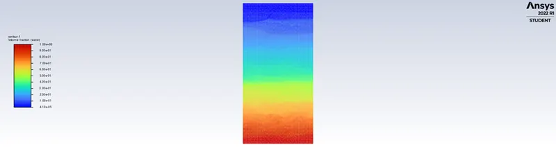
The phase contour is

https://youtu.be/HF6-eVbS9Dc

ATWOOD NUMBER (A):

The Atwood number (A) is a dimensionless number in fluid dynamics used in the study of hydrodynamic instabilities in density stratified flows.It is a dimensionless density ration defined as

`A=(rho1-rho2)/(rho1+rho2)`

where `rho1` is density of heavier fluid

`rho2` is density of lighter fluid

For case-I and Case-II (fluid water and air)

`rho1` = Density of water = 998.2 Kg/m3

`rho2` = Density of air = 1.225 Kg/m3

A=0.9975

For Case-III (fluid water,air and user material)

`rho1` = Density of water = 998.2 Kg/m3

`rho2` = Density of user material = 400 Kg/m3

A=0.427

For A close to 0, RT instability flows take the form of symmetric 'fingers' of fluid.

For A close to 1, the much lighter fluid goes below the heavier fluid that takes the form of larger bubble like plumes.

CONCLUSION:

In the above simulation results it starts with the state of hydrostatic equilibrium, and the Rayleigh Taylor instability is observed at the interference when a low density fluid pushes a high density fluid due to which formation of shock waves at the interface takes place. Formation of air bubbles starts taking place which compresses the heavy fluid around it, due to which shock waves of multidimensional fashion generates and it gets more stronger as it moves upwards.

It is observed that the more we refine the mesh the more simulation results get smoother about the irregularities that take place at the interface of the two fluids. As higher density fluid replaces lower density fluid, the formation of air bubbles and vortex takes place, which travels towards the upward region with time.

In case-III we see more detail results about the formation of waves and the formation of some air bubbles that get trapped at the lower region during the initial stage and then they travel towards the upper region, generating shock waves. At the end of the simulation, it is observed that two phases get separated from each other though, we can see some diffusivity between them which is a volume fracion of air and water.

In Rayleigh Taylor instability, due to sudden collapse in the layer between the denser and lighter fluid spike generation takes place which is obviously time dependent, hence using a steady state solver will not work as we are interested in the flow parameters with respect to time.

Google drive link Gdrive link