Week 5 - Rayleigh Taylor Instability

Aim –

To Simulate the Rayleigh Taylor instability using two different fluids for different mesh size.

Introduction –

1. The Rayleigh Taylor is phenomena that occur at the interface of two fluids of different density. In this heavier fluid pushes the lighter fluid.
2. Examples include the behaviour of water suspended above oil in the gravity, supernova explosions in which expanding core gas is accelerated into denser shell gas etc.
3. Models which capture the Rayleigh Taylor instability accurately in CFD are K-L turbulence, diffuse approximated methos and volume of fluid method. These models solve the governing equation of volume fraction, momentum and other equation using implicit or explicit approach.

Geometry –

Design the geometry in space claim as shown below. Both rectangles are of same size 20mm x 20mm.

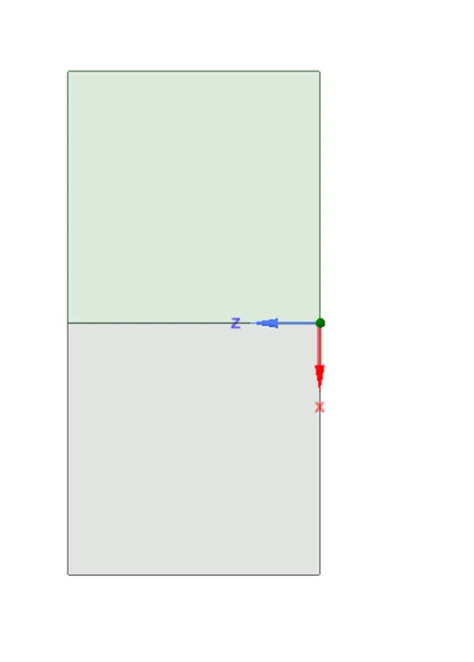
Case 1 - For simulation we will use two size of grid 0.5mm and 0.25mm . and do the simulation study of the raleigh taylor instability phenimena.

1. Mesh size - 5 mm

Import the geomtery in the meshing tab, generate the base mesh size of 0.5 mm .

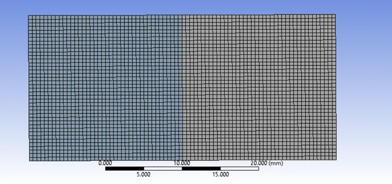
Setup

Solver Type – Pressure based and Transient

velocity formulation – Absolute

Tick marks the gravity and define the gravitational acceleration as - 9.81 m/sec.

Fluid type – Fluid 1 - Air, Fluid 2 - Water

Model – Viscous – Laminar

Multi-phase model – Volume of fluid

Volume fraction parameters – Implicit

No of Eulerain phases – 2

Interface modelling – Sharp

Phases – Air – Primary phase

Water – Secondary phase

Initialization – Hybrid

Patch - After initialization is set patch the phases. Enter the volume fraction 1 for the water and 0 for the air.

Time step size – 0.001 sec

Time steps – 500 sec

Outputs -

Residual plot

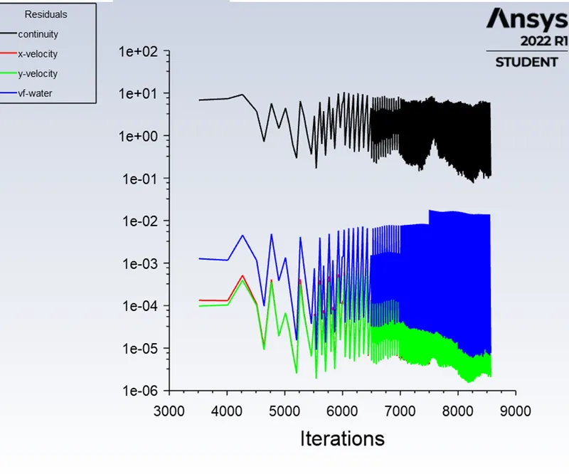
Animation-

https://youtu.be/1uVvCawqwdg

2. Mesh size - 0.25 mm

Generate the mesh size of the 0.25 in meshing tab. Rest the setup is same as of mesh size 0.5mm settings.

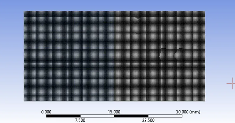
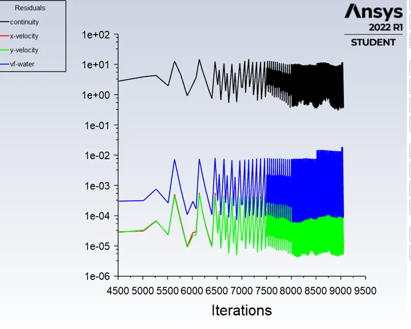
Outputs -

Residual plot

Animation link -

https://youtu.be/MmzwLks1da4

Case 2 -

In this we do study water and user defined material with properties shown below.

User-defined material – Density = 400 kg/m3

Viscosity = 0.001 kg/m-

Mesh size is taken for this simulation is 0.25mm and rest the setup setting will be same as above.

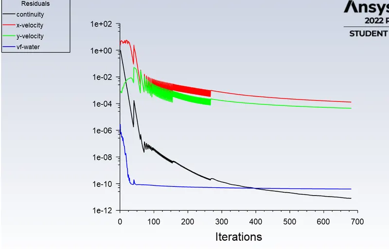
Results –

Residual plot

Conclusion –

1. It is observed from the results the finer the meash size give better capturing data to understand the displacement of fluids. It also take longer to get stability.
2. In coarser mesh the heavy fluids settle very fast.
3. The larger time step also lead to the floating point exception error due to arthmetic operation.

Transient state over steady state –

When the interface between two fluid is collapse the instability among the fluid is generated, this all is time time dependent.These changes are difficult to resord in the steady state solver .

Atwood Number- The Atwood number (A) is a dimensionless number in fluid dynamics used in the study of hydrodynamic instabilities in density stratified flows. It is a dimensionless density ratio defined as

P1 - density of heavier fluid

P2 - density of lighter fluid

Case 1 -

density of heavier fluid – 998.2

density of lighter fluid - 1.225

A =998.2 – 1.225 / 998.2 + 1.225

A = 996.975 / 999.425= 0.9975

Case 2 -

density of heavier fluid – 998.2

density of lighter fluid - 400

A =998.2 – 400 / 998.2 + 400

A = 598.2/1398.2 = 0.4278

In case 1 th value of Atwood no is 0.9975 , in this case th formation of bubble and spike will occur .

The range of atwood no from 0 -1 indicate the bublle formation with different density difference.