Week 5 - Rayleigh Taylor Instability
OBJECTIVE: To perform Rayleigh-Taylor Instability Simulation.
THEORY:
Rayleigh-Taylor Instability is a phenomenon that occurs at the interface of fluids of different densities where the fluid with lower density pushes the fluid with higher density due to the difference in density. It is a dynamic process where the system tries to reduce its total potential energy to attain the steady state point.
The system is in hydrostatic equilibrium at the initial stage of the process, here the high-density liquid is on top or above the low-density liquid in the container.
Some real-life examples are water suspended atop oil, supernova, and mushroom clouds formed due to volcanic eruptions.
Practical CFD models based on the mathematical analysis of Rayleigh-Taylor waves are;
Ritchmyer-Meshkov Instability: RMI arises when a shockwave interacts with an interface separating two different fluids.
Plateau-Rayleigh Instability: PRI explains the falling of a stream of fluid and it’s breaking down into smaller packets.
Kelvin-Helmholtz Instability: KHI occur when there is velocity shear in a single continuous fluid where there is velocity difference across the interface between two fluids.
The following mathematical model have been adapted for certain CFD calculations which involve
Smoother particle hydrodynamics: SPH is a computational method used for simulating the mechanics of continuum media such as solid mechanics and fluid flows.
Single-fluid Model: Here the individual phases are assumed to be flowing mixture described in terms of mixture properties.
Two-fluid model: Here separate sets of governing equations for the vapor and liquid are used.
PROCEDURE:
GEOMETRY
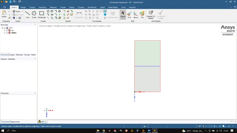
We start by opening space-claim in Workbench and create a square of 20*20mm after which we use pool tool to convert the sketch into a surface, after that we name the surface as air and add a new component to the main design after which we go into sketch mode and create a 20*20mm square right above the previous one and name it water. Now we head to the workbench section where we use the share tool to share the topology of both the surfaces in order to generate conformal mesh during meshing.
MESHING
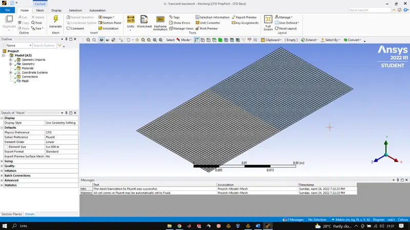
Meshing process is simple for this project we simply load the geometry and go to mesh and generate mesh and set the element size as 0.5mm as the geometry is small and simpler, we can refine the mesh even further but 0.5mm is perfect for a baseline simulation. Once the meshing is done we close the mesh GUI and head to the fluent setup.
SETUP(FLUENT)
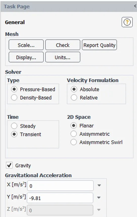
Transient time solver was selected and gravity was enabled in the Y- direction with value of 9.81m/s^2.
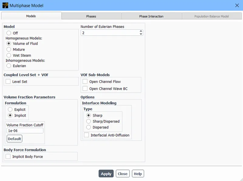
Multiphase simulation was setup and volume of fluid method was selected and the Implicit form was used for solving. Once this was done, we head towards phase and name our phases over there and select their element as well this is important as it will be needed for patching. Before this we should copy water-liquid from ANSYS fluent database so that we can have it as a matrial.
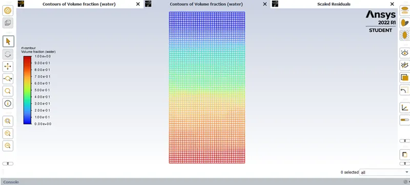
Once all this is done, we initialize by standard method and upon completion of initialization we go to patching to patch the surface with respective element. To check if our patching is right or wrong, we can plot a contour of the water phase over all the surfaces of the mesh if all the points above the half are red representing value 1 and lower half blue representing the value 0 our patching is correct, after verifying the patching we use create animation to create the solution animation and then run our simulation for time step size of 0.005 and number 550.
RESULTS:
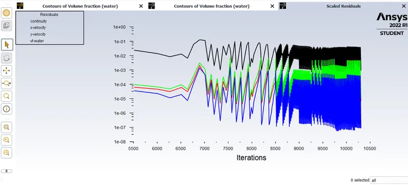
MESH ELEMENT SIZE 0.5MM
MESH ELEMENT SIZE 0.2MM
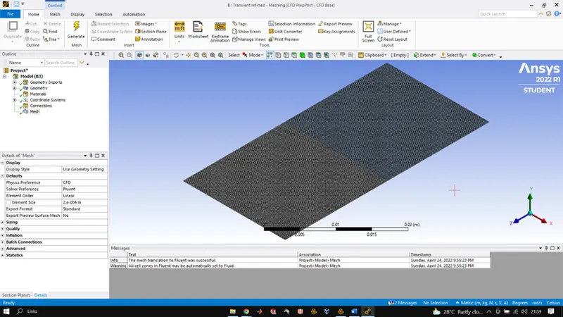
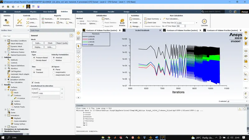
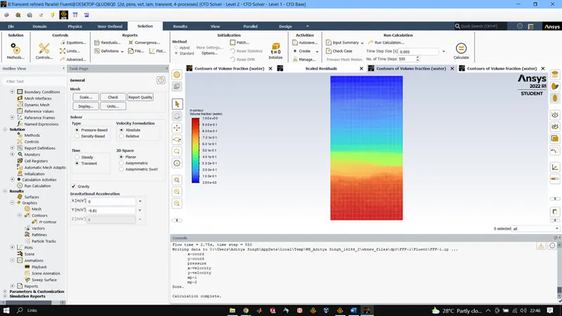
MESH ELEMNT SIZE 0.2MM WITH USER MATERIAL
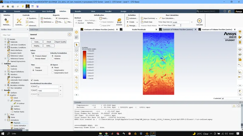
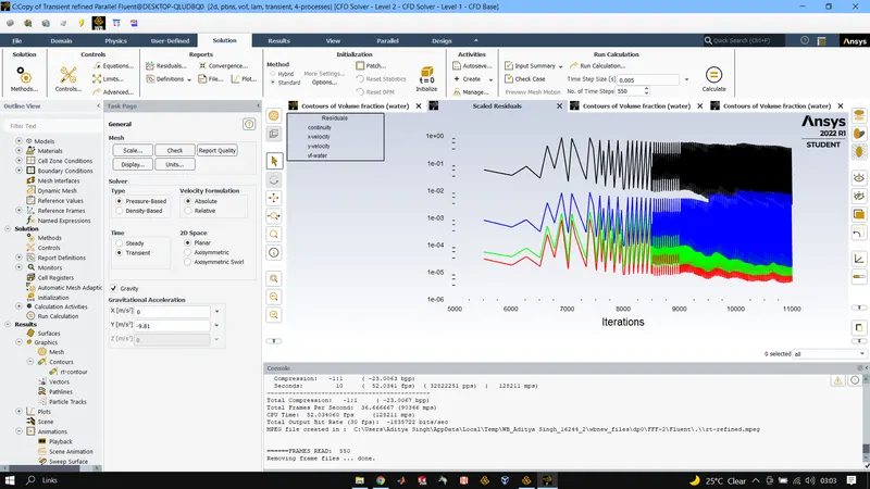
Atwood number (A) is a dimensionless number in fluid mechanics used in study of hydronamic instabilities.
`A = (rho1 - rho2)/(rho1 + rho2)`
`A = (997-1.225)/(997+1.255) = 0.9975 for Air-water case`
`A = (997 - 400)/(977 + 400) = 0.4275 for User material - water case`
CONCLUSIONS:
The finer mesh is able to capture the instabilities more efficiently than the base mesh but it also takes more time for the simulation to run.
Here we want to see how the instabilities progress and how the heavier fluids settle hence transient method is preferred as it capture all the details of the path and the steady state only focus on the end results.
Atwood number is used for validation of CFD simulation, for Atwood number close to 0 RT instability takes form of symmetric fingers and when it is close to 1 we see larger bubbles as seen in case of air-water mixing.