Week 5 - Rayleigh Taylor Instability

Aim : To simulate Rayleigh Taylor Instability.

Theory :

Rayleigh Taylor instability is a phenomenon that occurs at the interface of fluids of different densities wherein the lighter fluid pushes the heavier fluid due to the density difference. it is a dynamic process wherein the system tries to reduce its combined potential energy.

From the Newton's law of viscosity, we know that the fluid cannot resist even the lightest shear force. Density is one of the main properties of the fluid which the shear force can incorporate with it.

Depending upon the density we have lighter fluid like water etc and denser fluid like mercury, oil, honey etc.

Lord Rayleigh observed that when two fluids. i.e., lighter and heavier fluids are mixed together where the denser fluid is at top of the lighter fluid, due to the gravity and the density variation in the interface of the fluid is not stable. i.e., water suspended on the oil.

So, the instability of the interface between the different densities of fluid when the lighter fluid is accelerated towards the heavier fluid is known as Rayleigh Taylor Instability.

CFD models based on mathematical analysis of Rayleigh Taylor waves :

• Richtmyer-Meshkov instability
  The Richtmyer-Meshkov instability arises when shockwave interacts with an interface separating two different fluids. It combines compressible phenomena, such as shock interaction and refraction with hydrodynamic instability, including the nonlinear growth and subsequent transition to turbulence across a wide range of Mach numbers.
• Plateau-Rayleigh instability
  The Plateau-Rayleigh instability, often just called the relay instability, explains why and how a falling stream of fluid breaks up into smaller packets with the same volume but less surface area. This fluid instability is exploited in the design of particular type of inkjet technology where by a jet of fluid is perturbed into a steady stream of droplets.
• Kelvin-Helmholtz instability
  It can occur when there is velocity shear in a single continuous fluid or where there is a velocity difference across the interface between two fluids. For example, a wind blowing over water, the instability manifests in waves on the water surface, more generally clouds, the ocean, Saturn bands, and the sun’s corona show this instability.

Solving and Modeling Approach :

A. Geometry

1. Open Spaceclaim.
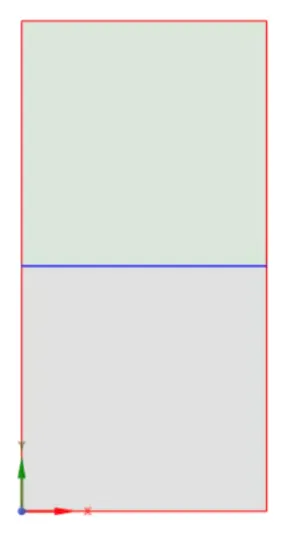
2. Use Rectangle tool and then create a rectangle from the origin.
3. Then use the Pull command to convert the rectangle to surface.
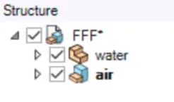
4. Then create a new component and again create another surface at the top the previous surface.
5. Then use Share tool to share the interface between both the surface.

B. Meshing

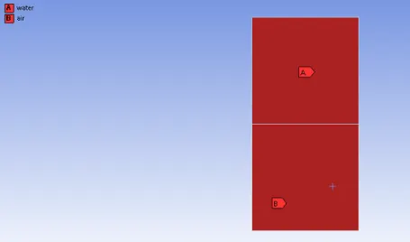
1. Open mesh and create the named selection to geometry upper square as Water and lower section as Air.
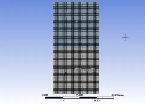
2. Mesh the geometry by using mesh size of 0.5 mm for basline mesh and 0.3 mm , 0.2 mm for refined mesh.
3. Close the mesh and update the mesh.

C. Setup

• General

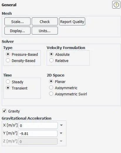
• Viscous Model we have used in the Case is Laminar for low velocity.
• Now, we have to check the Material Properties. In this study we have simulate the 3 cases. We have taken two Fluids Water and Air. The Heavy fluid at bottom is Water and the Lighter fluid at bottom is Air.
• Switch on Multiphase model and select Volume of fluid method

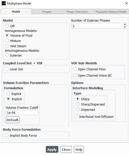
• Create the phases air as primary phase and water as secondary phase.
• Initialization of the model
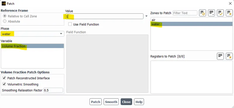
• Patching : After standard initialization, we need to patch both the respective materials, where we provide a volume fraction value of 1 for the water and 0 for the air and user defined material.

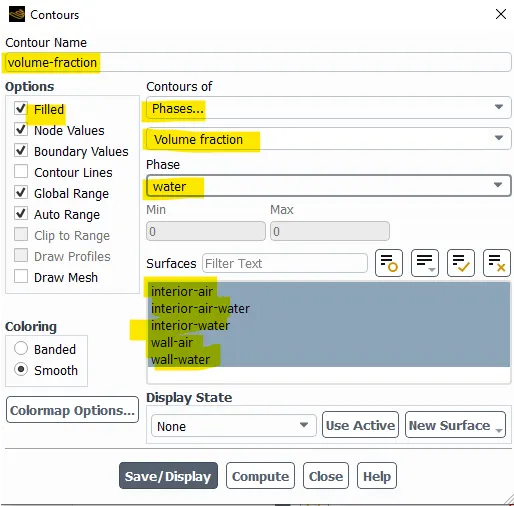
• Create a contour for the volume fraction.
  
• Create a animation for the result.
  
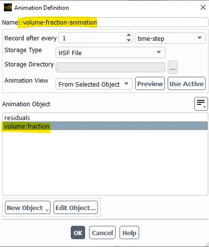
• Run calculation for 1500 time steps and size of time step is 0.005 sec.

Results :

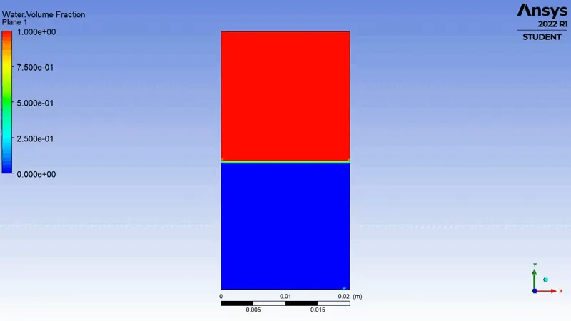
Case 1 : Baseline setup result of Air and Water (mesh size = 0.5 mm)

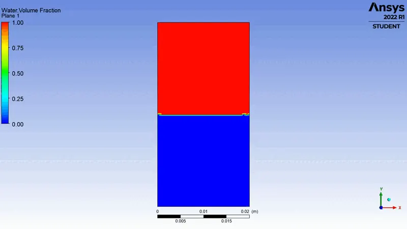
Case 2 : Refined mesh result of Air and Water (mesh size = 0.3 mm)

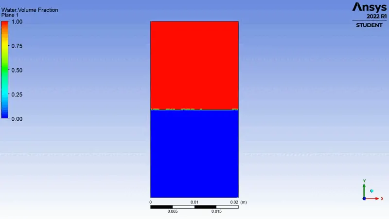
Case 3 : Refined mesh result of Air and Water (mesh size = 0.2 mm)

Case 4 : Refined mesh result of User-material and Water (mesh size = 0.2 mm)

User defined material of density = 400 kg/m³, viscosity = 0.001 kg/m-s

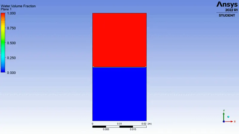
Animation File :

1. Baseline setup result of Air and Water (mesh size = 0.5 mm)

https://drive.google.com/file/d/16ecTKBaPZfJY_CLk0A537IiKLH3NWJXE/view?usp=sharing

2. Refined mesh result of Air and Water (mesh size = 0.3 mm)

https://drive.google.com/file/d/1dDd40636YON7umZqgTyrryajalUJz762/view?usp=sharing

3. Refined mesh result of Air and Water (mesh size = 0.2 mm)

https://drive.google.com/file/d/1lFx_tkEnzPB0I6Zf44WGVxdsxG_nhWkC/view?usp=sharing

4. Refined mesh results of User-material and Water (mesh size = 0.2 mm)

https://drive.google.com/file/d/1xdqZDKg9wJv7NQJqlg0cg7MJkhv3xpQd/view?usp=sharing

Conclusion :

• In all the cases, it was observed that fluid was starting to diffuse quit symmetrically, but once the air/use define material bubble was touching the top surface it was becoming distorted. Finer meshes captures the instability better than coarse mesh, but it takes more time to for the heavier fluid to settle down. it is computationally expensive but produces results with better accuracy.

• From the above Animations we can observe that Finer Mesh element size 0.2mm Captures the instability better than the coarse mesh element size 0.5 mm and As we see the heavier fluid takes more time to settle down as compared to the lighter fluid.

• In the Simulation we can clearly see that the state of hydrostatic equilibrium and the RTI is observed at the Interface when the lower density fluid is pushed by the heavy density fluid due to which the formation of the shock waves at the Interface takes place. Formation of air bubbles starts taking place, which compresses the heavy fluid around it, due to which shock waves of multidimensional fashion generates and it gets more stronger as it moves upward.

• As we fine the mesh more the simulation results gets more smoother about the irregularities that takes place at the Interface. As higher Density Fluid replaces the lower density air bubbles are formed and also vortex formed, which travels towards the upward region with time.

• At the end we can clearly see that two phases gets separated from each other and settle down though we can see diffusivity between them which is a volume fraction of water.

Why a steady-state approach might not be suitable for these types of simulation ?

As we know In Steady state simulation is preferred to concern more about the final results or the equilibrium state and also you cant see the small-time variation of instability. In RT instability CFD models, we are more concerned to learn about the transition of the irregularities that starts devolping when heavy and low densities fluids mixing under the effect of gravity So, by using the Transient state solver with the refined mesh we can compute the smooth Transition of irregularities takes place at the Interface of the two Fluids.

But the Final state of Steady and Transient State solver must be same and We want to see the behaviour of the solution at every instant of time such that capturing of bubbles, shock-waves, vortex. So, we prefer Transient state solver to see the RT instabilty.

Concept of Atwood number in RTI :

The Atwood number (A) is a dimesionless number in fluid dynamics used in the study of hydrodynamic instabilities in density stratified flows. It is a dimensionless density ratio defined as

`A =( rho_1-rho_2)/(rho_1+rho_2)`

where

`rho_1` = density of heavier fluid

`rho_2` = density of lighter fluid

Atwood number is an important parameter in the study of Rayleigh–Taylor instability. In Rayleigh–Taylor instability, the penetration distance of heavy fluid bubbles into the light fluid is a function of acceleration time scale, `Ag t^2` where g is the gravitational acceleration and t is the time.

Variation in Atwood number in the above cases affects the behavior of the instability :

RTI envloves in three disctinct stages: linear stability, bubble Formation, long term evolution due to bubble merging and mixing. When A >0.5 RTI mixing and is shown to recover important statistical measures of the mixing process, such as bubble and spike growth rates and mixing efficiency reported in that study, but at the significantly coarser resolutions typical of most large-eddy simulations.

The simulations of RTI at Atwood numbers A > 0.9 then used to explore the effects of varying the density ratio on mixing dynamics at very high Atwood numbers 0.75 > A >0.95. Spike heights and mixing layer growth rates are shown to be strongly affected by the initial density ratio. An empirical power-law scaling relationship is shown to predict nearly exactly the variation in the ratio of spike to bubble heights as a function of Atwood number.