Week 5 - Rayleigh Taylor Instability

Aim: To conduct the Rayleigh-Taylor Instability analysis.

Objectives:

Draw 2-D geometry in the Ansys-Space claim and conduct transient simulations on Ansys-Fluent for Rayleigh-Taylor Instability (RTI) for different meshes and densities. Below the following objectives are to present in the report.

1. What are some practical CFD models that have been based on the mathematical analysis of Rayleigh Taylor waves? In your own words, explain how these mathematical models have been adapted for CFD calculations.
2. Perform the Rayleigh Taylor instability simulation for 2 different mesh sizes, with the base mesh being 0.5 mm. Compare the results by showing the animations (Attach them from your google drive). Observe the differences in the animation and explain the effect of mesh size on simulation. Also, explain why a steady-state approach might not be suitable for these types of simulation. [Choose Air and Water for this simulation]
3. Run one more simulation with water and user-defined material (density = 400 kg/m³, viscosity = 0.001 kg/m-s) for refined mesh.
4. Define the Atwood Number. Find out the Atwood number for both the cases and explain how the variation in Atwood number in the above two cases affects the behavior of the instability.

Rayleigh-Taylor Instability

Rayleigh-Taylor Instability (RTI) is a dynamic phenomenon that occurs at the interface when different density fluids are mixed, where the lighter density fluid pushes the heavy density fluid due to the density difference. In this process, both are mixed and tries to decrease the combined potential energy. RTI phenomenon includes integral boundary method, front tracking method, the volume of fluid methods, level set method and phase filed methods.

Physics behind RTI

In a constant gravitation field, the complete system is in hydrostatic equilibrium in which the heavy density fluid lies above the light density fluid. As RTI develops, the initial perturbations grow linearly and eventually create upward flowing “plumes” and downward falling “spikes” due to the interplay between buoyancy and gravitation. In the linear phase, equations can be linearized, and the amplitude of perturbations grows exponentially with time, while for the non-linear, perturbation amplitude is too large (neglected). In non-linear analysis, the density disparity between the fluid decides the structure of the flow.

Examples of RTI: Mushroom cloud after a volcanic eruption and atomic explosion, decoction and milk mixing, water-oil mixing etc.

Objectives

1. What are some practical CFD models that have been based on the mathematical analysis of Rayleigh Taylor waves? In your own words, explain how these mathematical models have been adapted for CFD calculations.

Practical CFD Models

1. Smoother Particle Hydrodynamics (SPH)

Smoother particle hydrodynamics (SPH) is a mesh-free particle method based on the Lagrangian formulation (where the coordinates move with the fluid), and the resolution of the method can easily be adjusted with respect to variables such as density. This computational approach is used to simulate the mechanics of continuum media, like solid mechanics and fluid flow. It is also used to model fluid motion as well. In SPH, the particles themselves represent, so it guarantees conservation of mass without extra computation effort. SPH computes pressure from weighted contributions of neighboring particles rather than by solving linear systems of equations. SPH creates a free surface for two-phase interacting fluids since the particles represent the denser fluid and space represent the lighter fluid. For these reasons, it is possible to simulate fluid motion using SPH in real-time.

2. Single Fluid Model

The applied single-fluid model is a five-equation model consisting of the mass, momentum and energy equations for a vapour/liquid mixture and two equations describing the formation and growth of the liquid phase.

3. Two-Fluid Model

Two-fluid models are termed Eulerian–Eulerian models because both the particulate and the gaseous phase are considered continuous, fully interpenetrating continua coupled by an interaction term. The two-fluid model solves two sets of equations governing, i.e.; the conservation of mass, momentum and energy.

4. Turbulence Model

The turbulence model predicts the average mixing behaviour in the flow on average one or two dimensional. The two-equation K-L turbulence model involves the equation of turbulence kinetic energy (K) and turbulent length scale (L), whereas the three equation K-L-a turbulence model includes turbulence mass flux velocity as a third turbulent equation.

2. Rayleigh- Perform the Rayleigh Taylor instability simulation for 2 different mesh sizes, with the base mesh being 0.5 mm. Compare the results by showing the animations (Attach them from your google drive). Observe the differences in the animation and explain the effect of mesh size on simulation. Also, explain why a steady-state approach might not be suitable for these types of simulation. [Choose Air and Water for this simulation]

Model Preparation

The geometry consists of 20 mm x 20 mm squares, one on the top other as shown in Fig. 1. The top square is named “water” and below as “Air”. The common edge between the domain is shared using the shared tool.

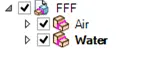
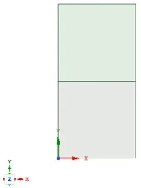
Fig 1. Geometry

Simulation details:

A transient state simulation is carried out using Pressure based solver. For laminar viscous model has been used. Water and air are defined as the multiphase fluid flow domain. The volume of fluid (VOF) model with an explicit approach is used. Air is taken as the primary phase and water as the secondary phase.

Case 1-Base line Mesh

Element size=0.5 mm

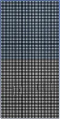
Fig. 2 Mesh

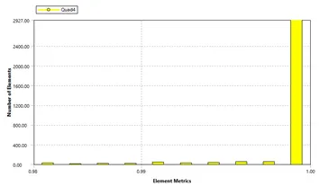
Fig. 3 Mesh metric

Animation video link of 0.5 mm Mesh:

Case-II (Refine Mesh)

Element size= 0.25 mm

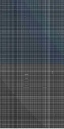
Fig. 4 Mesh

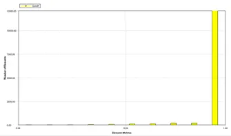
Fig. 5 Mesh metric

Animation video link of 0.25 mm Mesh (refine mesh):

Observations

In all the above cases, it is observed that the simulation starts with the hydrostatic equilibrium and Rayleigh Taylor instabilities are found at the interface when light density fluid pushes the high-density fluid due to which formation of shock waves takes place the interface. The formation of light density fluid bubbles compresses the high-density fluid around it, due to which multidimensional shock waves propagates and get stronger as it moves upward.

As we more refine the mesh, finer mesh capture instability more accurately than coarse mesh but takes more time for the computational simulation. Diffusivity of different densities fluid can be easily found in the refined mesh.

Why might a steady-state approach not be suitable for these types of simulation?

Transient simulation gives the variation of a phenomenon with respect to time. While steady-state simulations have opted when we are looking for the final results only. In RT instability, we are more concerned about the interfacial irregularities happening due to mixing two different fluid densities. Transient simulation with refined mesh gives detail of irregularities like bubble formulation, vortex, and shockwaves at the interface of the fluids. So, this reason for choosing transient simulation over steady-state simulation.

3. Run one more simulation with water and user-defined material (density = 400 kg/m³, viscosity = 0.001 kg/m-s) for refined mesh.
4. 

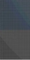
Fig 6. Mesh

Animation video link of 0.25 mm Mesh (refine mesh) for Water-User defined fluid:

4. Define the Atwood Number. Find out the Atwood number for both the cases and explain how the variation in Atwood number in the above two cases affects the behaviour of the instability.

The Atwood number (A) is a dimensionless number in the fluid dynamics used to study hydrodynamic instabilities in density stratified flows. It is a dimensionless density ratio defined as follows.

Where `ρ1`=density of the heavier fluid.

ρ2=density of the lighter fluid.

In Rayleigh–Taylor instability, the penetration distance of heavy fluid bubbles into the lighter fluid is a function of acceleration time scale, Agt² where g is the gravitational acceleration and t is the time.

Atwood number in Case-I and Case-II

ρ₁₌998 kg/m³ (water)

ρ₂₌1.25 kg/m³ (Air)

Atwood number in Case-III

ρ₁₌998 kg/m³ (water)

ρ₂₌400 kg/m³ (User define fluid)

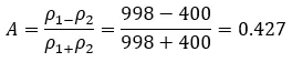
When Atwood number is close to zero (0), instability takes the form of symmetric ‘finger’ of fluid, whereas Atwood number 1 lighter fluid takes the form of large bubble-like plumes. Rayleigh Taylor Instability evolves in three distinct stages, (i) Linear stability (ii) Bubble formation (rising) or Mushroom head formation (falling) and (iii) long term evolution due to mixing and merging. At low Atwood number, bubble or mushroom head formation are symmetric in nature and the perturbation/disturbance are linear for a larger time. In contrast, for larger Atwood number heads are not symmetrical and it occurs very fast at an accelerating rate which eventually leads to non-linear growth.

Conclusions

1. Formation of bubble and mushroom-like structures.
2. In 0.5 mm mesh, large disturbances are found at the water-air interface it forces high-density fluid-like shock wave.
3. In 0.25 mm mesh, less disturbances are found and mushroom-like structure is found around the high-density fluid.
4. At higher Atwood number, more instabilities are found and measuring of spike of instability is very difficult.
5. Low Atwood number shows linearity and stable flow of mixture.