Week 5 - Rayleigh Taylor Instability

Objective

1. What are some practical CFD models that have been based on the mathematical analysis of Rayleigh Taylor waves? In your own words, explain how these mathematical models have been adapted for CFD calculations.
2. Perform the Rayleigh Taylor instability simulation for 2 different mesh sizes with the base mesh being 0.5 mm. compare the results by showing the animations (Attach them from your google drive). Observe the differences in the animation and explain the effect of mesh size on simulation. Also, explain why a steady-state approach might not be suitable for these types of simulation.[ Choose Air and Water for this simulation]
3. Run one more simulation with water and user-defined material (density = 400 kg/m³, viscosity = 0.001 kg/m-s) for refined mesh.
4. Define the Atwood Number. Find out the Atwood number for both the cases and explain how the variation in Atwood number in the above two cases affects the behaviour of the instability.

Rayleigh Taylor Instability

The Rayleigh Taylor instability is an instability of an interface between two fluids of different densities (heavy fluid at the top and lighter fluid at the bottom) due to buoyancy of lighter fluid pushes the heavier fluid (consider an 1^st quadrant of xy plane buoyancy acting +y direction upwards) the gravitational field and surface tension of lighter fluid would be acting downward direction (-9.81m/s²) due to these there would be an disturbance/ instability in the medium

When the density interface is disturbed, the hydrostatic pressure is generated, so the heavier fluid moves downwards and mixes with the lighter one, with the amplitude of perturbation initially growing exponentially but after sometime saturates and forms characteristic mushroom shape. When a heavier fluid is displaced downward with an equal volume of lighter fluid displaced upwards, it results in decrease of potential energy than its initial state. This RTI has been applied to a wide range of problems including the mushroom clouds like volcanic eruptions, nuclear explosions and plasma fusion reactors instability

Types of instabilities and some practical CFD models that have based on mathematical analysis of Rayleigh Taylor waves

1. Plateau–Rayleigh instability

The Plateau–Rayleigh instability, often just called the Rayleigh instability, explains why and how a falling stream of fluid breaks up into smaller packets with the same volume but less surface area. It is related to the Rayleigh–Taylor instability and is part of a greater branch of fluid dynamics concerned with fluid thread breakup. This fluid instability is exploited in the design of a particular type of ink jet technology whereby a jet of liquid is perturbed into a steady stream of droplets.

2. Kelvin–Helmholtz instability

The Kelvin–Helmholtz instability (after Lord Kelvin and Hermann von Helmholtz) typically occurs when there is velocity shear in a single continuous fluid, or additionally where there is a velocity difference across the interface between two fluids. A common example is seen when wind blows across a water surface; the instability constant manifests as waves. Kelvin-Helmholtz instabilities are also visible in the atmospheres of planets and moons, such as in cloud formations on Earth or the Red Spot on Jupiter, and the atmospheres

3. Richtmyer–Meshkov instability

The Richtmyer–Meshkov instability (RMI) occurs when two fluids of different density are impulsively accelerated. Normally this is by the passage of a shock wave. The development of the instability begins with small amplitude perturbations which initially grow linearly with time. This is followed by a nonlinear regime with bubbles appearing in the case of a light fluid penetrating a heavy fluid, and with spikes appearing in the case of a heavy fluid penetrating a light fluid. A chaotic regime eventually is reached and the two fluids mix. This instability can be considered the impulsive-acceleration limit of the Rayleigh–Taylor instability

Geometry setup

At first, geometry is created, 2 square box of 20*20 bottom contains the lighter fluid and top contains heavier fluid for both square boxes we use pull option to make a surface then both boxes are selected they are shared –share option due to which share topology will turned on

Meshing

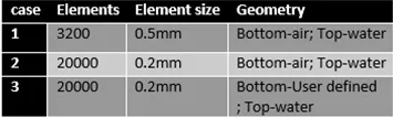
Case setup

1. Pressure based solver and Absolute velocity is used.
2. Transient-state Calculation is performed.
3. Compressible fluid flow is chosen.
4. Gravity is enabled in -ve Y axis
5. Multiphase Model is turned on along with Volume of Fluid and number of Eulerian phases is chosen as 2 and implicit scheme is selected.
6. Viscous model-Laminar is used.
7. Cell zone selected as Fluid-air;water-surface:water-liquid
8. Patching of the volume fraction of the two phases is performed before the start of simulation. Phase used for patching was water and volume fraction of 1 is taken for water surface and 0 for air surface.
9. In Pressure velocity coupling SIMPLE scheme is used. For the momentum second order upwind scheme is used and for pressure, PRESTO is selected. For the transient formulation first order implicit scheme is chosen

Solution animation

Case1:

https://drive.google.com/file/d/11qZ9PJPyWlSAmCZq1WOL6LKHVQ9xMBva/view?usp=sharing

Case2:

https://drive.google.com/file/d/11nzkQf5GUfFJslg6Kh2JB0sykJ3F9WyJ/view?usp=sharing

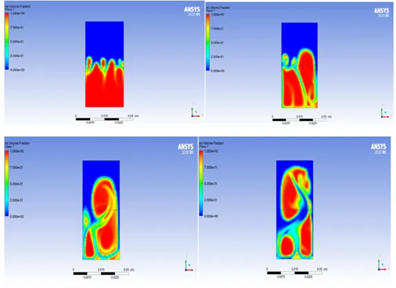
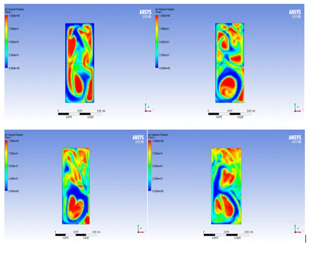
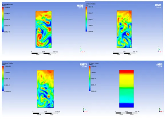
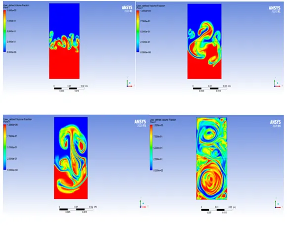
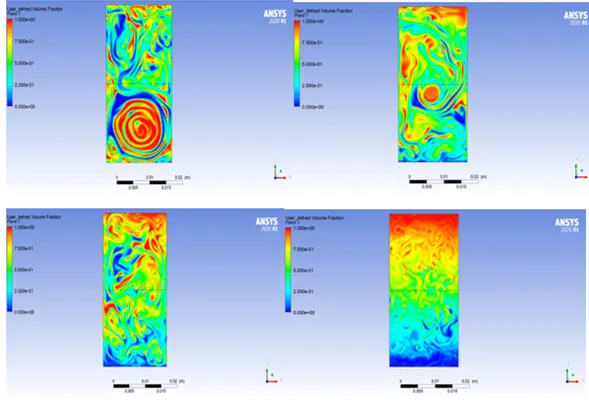
Contour plots at different time step of case 1

Observation

• The animation clearly suggests that higher the mesh resolution better will be physics being captured by the model
• We can’t use steady state approach here because each time step is crucial to determine change in state of the model (when the heavier fluid moves downwards and mixes with the lighter one, with the amplitude of perturbation initially growing exponentially) which only be captured by transient state

Case3:

https://drive.google.com/file/d/11ro2nCRxYQWikxPc_dGVIvqjuNbL0l5m/view?usp=sharing

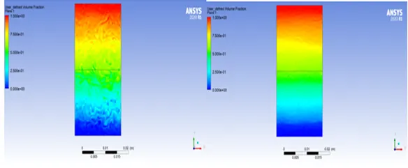
Contour plot at different time step case3

Atwood number

The Atwood number is a dimensionless number in fluid dynamics used in the study of hydrodynamic instabilities in density stratified flows. It is a dimensionless density ratio related to the density of heavier fluid and the density of lighter fluid. (The difference in the fluid densities divided by their sum).

A =`(rho_1-rho_2)/(rho_1+rho_2)`

ρ₁= density of heavier fluid;

ρ₂= density of lighter fluid;

Case1 and Case 2: For fluid materials air and water

ρ₁= density of water =998.2kg/m³;

ρ₂=density of air= 1.225kg/m³;

A= (998.2-1.225)/ (998.2+1.225) = 0.9975 ≈ 1(rounding off) ;

Case3: For fluid materials user defined and water

ρ₁= density of water =998.2kg/m³;

ρ₂=density of user defined= 1.225kg/m³;

A= (998.2-400)/ (998.2-400) = 0.427 ≈ 0 (rounding off);

Atwood number is an important parameter in the study of Rayleigh–Taylor instability. For Atwood number close to 0(case 2), RT instability flows take the form of symmetric “fingers” of fluid; for Atwood number close to 1(case 1), the much lighter fluid “below” the heavier fluid takes the form of larger bubble-like plumes.

Conclusions:

• Finer the grid size better will it be to capture the simulation undergoing the changes
• If Atwood number ≈ 1 simulation takes the form of larger bubble-like plumes and Atwood number ≈ 0 simulation takes form of symmetric “fingers” of fluid