Week 5: Project : Centrifugal pump simulation

CENTRIFUGAL PUMP SIMULATION:

Aim: To carry out a simulation of Liquid flow inside a Centrifugal Pump using Converge 3.0 CFD program and then post-process the results on Paraview.

Introduction: We need to observe the parameters of Water (H₂O) as a medium flowing inside a Centrifugal Pump. In this simulation we can examine the effects of rotation of the Impeller due to inflow of fluid with specific mass flow rate.

Theory: A Centrifugal pump is a mechanical machine that pumps the fluids by converting the mechanical power (rotational energy) into the pressure energy of the fluid flow. This mechanical power generally supplies by the electric motor or engine. A centrifugal pump uses a centrifugal force to pump the fluids. Therefore, it is known as a centrifugal pump.

The centrifugal pump working principle is according to the basic principle of the angular momentum principle which states that the change in the angular momentum of a revolving element is equivalent to the applied force. It represents, when a specific quantity of the fluid rotates due to an external force (force provide by an electrical motor or a turbine), a centrifugal force appears on the fluid, which further converts the fluid speed into pressure. Some part of this energy converts into the fluids’ kinetic energy.

The other parameters to be observed are change in the velocity, pressure, mass flow rate through-out the flow and total cell count.

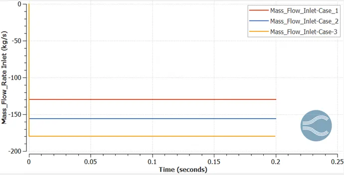
We used three different Mass Flow rates to run the simulation, which are as below:

• Case 1: Mass Flow Rate = 130 Kgs
• Case 2: Mass Flow Rate = 156 Kgs
• Case 2: Mass Flow Rate = 180 Kgs

Geometry:

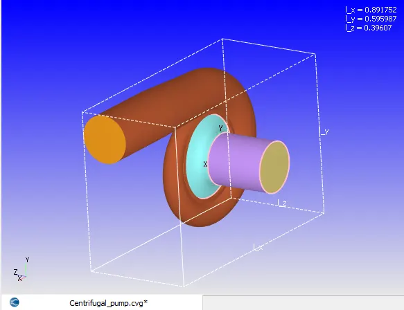
- In the Converge Studio first we import the ‘STL’ file of the geometry.

- Then, we carry out a ‘Diagnosis’ on the shape created to check for any errors. If there is no error then the geometry is correct.

- Then we move to case set up.

Case Set up Procedure:

- Application Type: Time-based

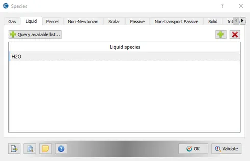
- Material: - Select Liquid Simulation & Species.

- Simulation Parameters:

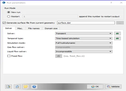
- Run Parameter: Transient Solver used to perform with Full Hydrodynamic mode with Incompressible Liquid flow Solver.

- Simulation Time Parameter:

- Start Time = 0 second

- End Time = 0.2 second.

- Initial Time Step = 1e-9 seconds

- Minimum Time Step = 1e-9 seconds

- Maximum Time Step = 1 second

- Maximum Convection CFL limit = 1

- Solver Parameters:

- Navier-Stokes Solver Type = ‘Density based’ selected.

- Misc. Setting:

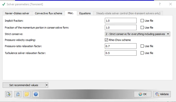
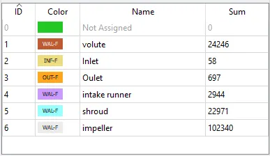
- Boundary Conditions:

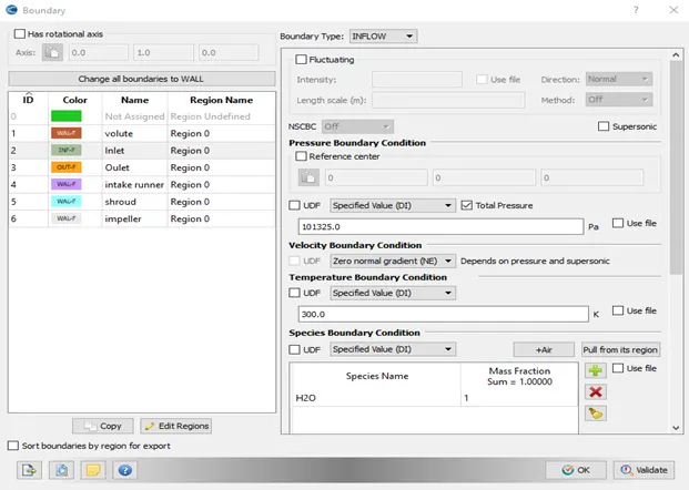
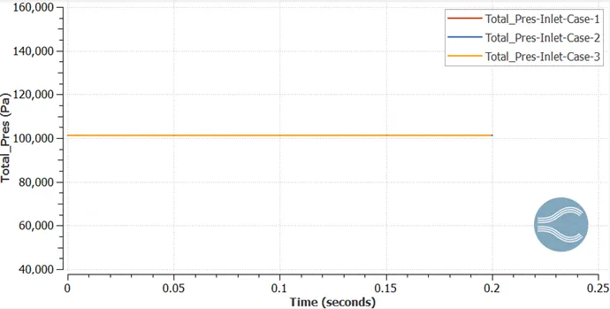
- Inlet: Inlet Pressure = 101325 Pa & Species Boundary Condition = H₂O (Mass Fraction = 1)

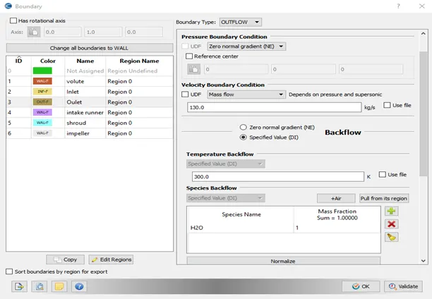
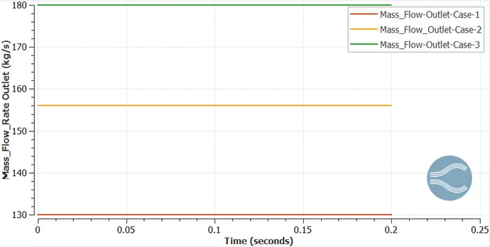
- Outlet: Outlet Mass flow – Case-1 = 130 kgs; Case-2 = 156 Kgs; Case-3 = 180 Kgs.

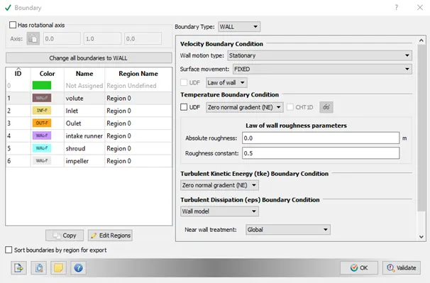
- Volute Boundary condition: Law of the Wall Condition.

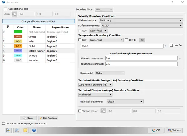
- Intake Runner Boundary Condition: Law of the Wall Condition.

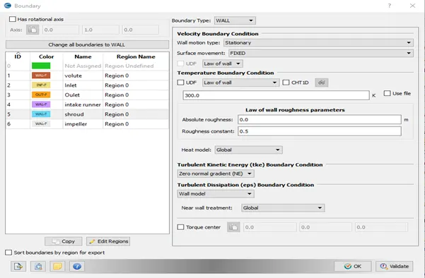
- Shroud Boundary Condition: Law of the Wall Condition.

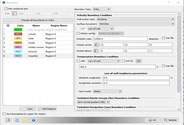
- Impeller Boundary Condition: Wall Motion= Rotating & Rotation rate = 12000 degree/s.

- Initial Conditions & Events:

- Regions: All boundaries defined to ‘Region 0’.

Initial Pressure = set to 101325 Pa; Temp. = 300 K.

- Species Mass Fraction: H₂O = 1.

- Physical Models:

- Turbulence Modelling= set to RANS [RNG K-Ɛ]

- Grid Control:

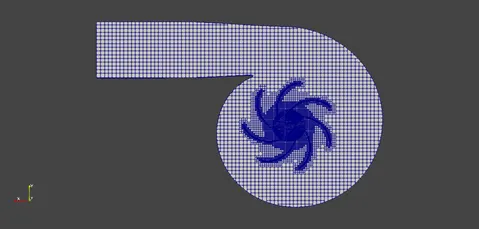
Base Grid Size: dx = dy = dz = 0.012 m

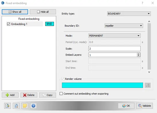
Fixed Embedding:

- Post Processing:

- Post variables Selection:

- Typical Variables/Geometry: Select desired variables such as Density, Velocity, pressure, temperature.

- Output Files:

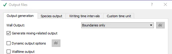
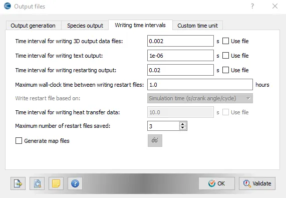
Case setup is complete with this.

- Export case setup: The case setup files are then ‘Exported’ to the destination folders to save the details.

- The destination folders should consist of following files in order to run the simulation and then post process the result on Paraview. The files are:

(i) converge.exe (name changed for the ease of run command on cygwin)

(ii) mpiexec.exe (name changed for the ease of run command on cygwin)

(iii) post_convert.exe (under output folder)

- Open Cygwin: Now the simulation is run using Cygwin. We navigate to the desired folder where the setup files were exported.

- Command to Run Simulation: The command to run simulation through Cygwin for Converge Studio 3.0 version is as below:

“ mpiexec.exe –n 2 converge.exe restricted “

• The simulation starts running, due to which output files are generated under a separate output folder.
• These output files are then post processed to convert the data in a format suitable for Paraview.

- Inline Plot: In the Converge Studio program, we can use Inline Plotting option to plot the curves during simulation run. We can observe the change in the plots and see the position of the simulation at the end of the time.

- Post Convert in Converge: To post process, we use file type as ‘Paraview VTK in-line binary format’. Now the files are post processed with a case name ‘test’.

- This generates ‘test.vtm’ group files which are generally used in Paraview to observe the results.

- Paraview: Open Paraview to check for the results.

Observations for All Cases:

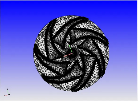
Mesh Formation = 130 Kgs.

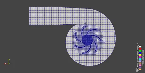
Mesh Formation = 156 Kgs.

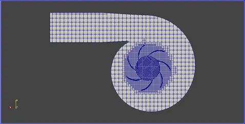
Mesh Formation = 180 Kgs.

Mass Flow Rate Plot - INLET:

Mass Flow Rate Plot - OUTLET:

Total Pressure Plot - INLET:

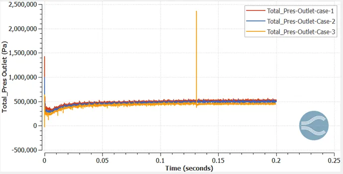
Total Pressure Plot - OUTLET:

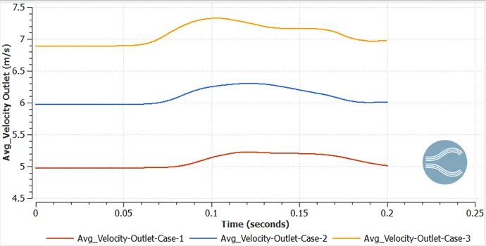
Average Velocity Plot - OUTLET:

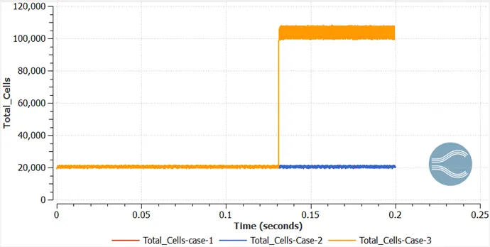
Total Cell Count:

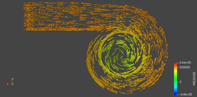
Pressure Glyph Contour:

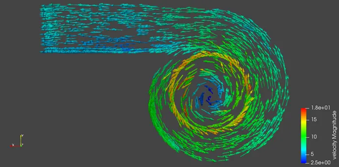
Velocity Glyph Contour:

Pressure-Velocity Animation: https://youtu.be/edYCPb3Mpo0

Wheel-Pressure Animation: https://youtu.be/N8VUpqQMGso

Results:

After running the simulation, the results can be observed as below:

• The Mass Flow rate Inlet & Outlet plots clearly show that the mass flow rate is conserved till the end.
• The Total Pressure at the outlet increases for all the three cases. For the mass flow rate of 180 Kgs the total pressure is somewhat less than the other two cases. This is due to increase in the friction with the increase in the velocity at the outlet.
• The Average Velocity plots depict that with the increase in the mass flow rate, the velocity at the outlet also increases 5 m/s, 6 m/s & 6.97 m/s respectively.
• The Total cell count for Case 1 & 2 remain same through-out the simulation i.e. about 20700, but for case 3 cell counts goes upto 1,00,000.
• From the pressure glyph contour and animation it is evident that the pressure is less at the inlet of the impeller and at the outlet pressure starts to rise due to spin of the impeller.
• From the velocity glyph contour and animation we can see that the velocity is high as the flow passes through the impeller and then it reduces as it strikes the volute. There is some flow separation observed as the flow area at the outlet increases. Later the flow smoothens due to longer length of the outlet casing.

Comparison of Total Pressure Vs Mass Flow Rate:

Particular	Mass Flow Rate (Kgs)	Total Inlet – Inlet (Pa)	Total Inlet – Outlet (Pa)
Case 1	130	101325	532179
Case 2	156	101325	505500
Case 3	180	101325	444011

Formula for Calculation of Pump efficiency:

Pump Efficiency = [Output Power / Input Power] x 100

Conclusion:

We can conclude from the simulation using Converge CFD program that:

• Simulation was run for three different Mass Flow Rates successfully.
• Simulation with coarse mesh sizes is sufficient to draw a conclusion about mass flow rate, pressure, velocity characteristics. But if we are supposed to capture the phenomenon of Cavitation, Slippage then we need to opt for finer mesh.
• The change in the parameters for a flow can be observed from the various animations, plots, contours and profiles.