Week 5: Prandtl Meyer Shock problem
AIM: 1. To do a literature survey on Shock Flows and its boundary conditions.
2. To describe the physics behind shock waves.
3. To observe the effect of SGS temperature value on cell count and the shock location
Introduction:
Shock Wave:
When the speed of the moving object in a medium becomes equal to the velocity of sound(340 m/s) in the medium, the wavefronts cannot escape from the source and pile up. This results in a large amplitude sound barrier. When the speed of the moving object or source exceeds the speed of sound in medium then the wavefronts lag behind the source forming a cone shaped region with a source at vertex. The edge of the cone forms a supersonic wave front with an unusually large amplitude called a shock wave. A sonic boom is heard when the shock waves reach an observer. The occurence of shock waves can be characterized by instantaneous change in pressure, velocity and temperature in a fluid flow. The region between the vehicle and the shock wave known as the shock layer will be a region of high pressure, density and temperature than the free-stream flow conditions. When a fluid streamline crosses the standing shock wave, abrupt increase in the pressure, temperature and density of the fluid flow occurs with a decrease in velocity of the flow.
Prandtl Meyer Shock Waves:
The normal shock waves are straight in which the flow before and after the wave is normal to the shock. It is considered as a special case in the general family of oblique shock waves that occur in supersonic flow. In general, oblique shock waves are straight but inclined at an angle to the upstream flow and produce a change in flow direction. An oblique shock generally occurs, when a supersonic flow is ‘turned into itself”.
Another class of two dimensional waves occurring in supersonic flow shows the opposite effects of oblique shock. Such types of waves are known as expansion waves . When the supersonic flow is “turned away from itself”, an expansion wave is formed. Here, the flow is allowed to pass over a surface which is inclined at an angle θ to the horizontal and all the flow streamlines are deflected downwards. The change in flow direction takes place across an expansion fan centered at point ‘A'. The flow streamlines are smoothly curved till the downstream flow becomes parallel to the wall surface behind the point ‘A'. Here, the flow properties change smoothly through the expansion fan except at point ‘A'. An infinitely strong oblique expansion wave may be called as a Mach wave . An expansion wave emanating from a sharp convex corner is known as a centered expansion which is commonly known as Prandtl-Meyer expansion wave.
In Prandtl-Meyer Shock Flow, supersonic waves are made to pass through the inlet of a duct that has a sharp corner. An infinite number of Mach Waves are created which spread out over a wide area or fan out creating a pattern that will be shown by simulating the flow in Converge Studio.
Boundary Conditions:
Boundary conditions used for shock flow problems are:
- Dirchlet BC: The value of the function is specified at the boundary. y = f
- Neumannn BC: The value of normal derivative of a function is specified. dy/dn = f
- Robin BC: Combination of both Dirchlet & Neumann. c0.y + c1.(dy/dn) = f
Neumann is used for supersonic outlets because the value of all parameters like pressure, temperature, velocity are not available before solving the problem. Nothing is specified at a supersonic outlet and all variables are extrapolated from the domain interior. Only the normal derivative of variables are specified as 0.
Geometry:
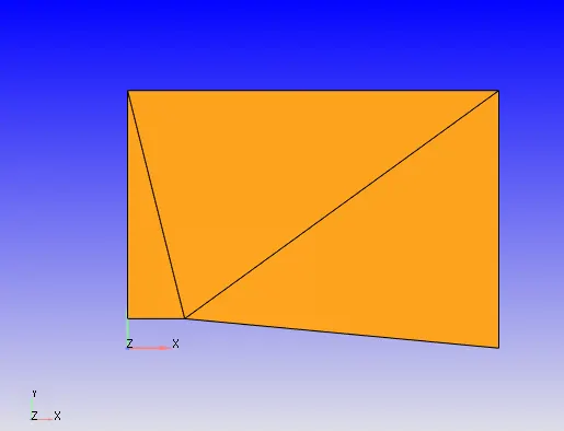
The following is the geometry used for the simulation of shock flow.
Case setup:
- Density based Steady state solver with full hydrodynamic and compressible solver for gas.
- Simulation time is 0 and end time upto 25000 cycles.
- Inflow, pressure BC is set to NE, velocity is of 680m/s.
- Outflow, pressure BC is set to NE.
- Front & Back are set to 2D.
- Top and bottom are selected as walls.
- Regions and Initialization: velocity = 680m/s, Temp = 300K, Pressure = 50000Pa.
- Turbulence modelling = RNG k-epsilon
- Base grid = 0.8m
- Adaptive Mesh Refinement is enabled with field variable as Temperature.
Results:
Case-1 : Velocity = 680m/s, SGS = 0.05
Case-2 : Velocity = 690m/s, SGS = 0.03
Case-3 : Velocity = 680m/s, SGS = 0.1
Case-1 : (Velocity = 680m/s, SGS = 0.05)
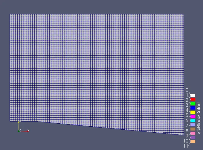
Since the mesh size is 0.8m for all cases the following is the generated mesh
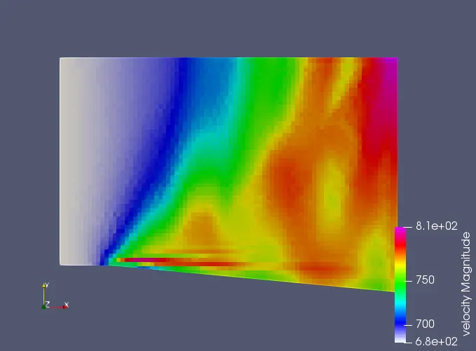
Velocity Contour:
Velocity plot:
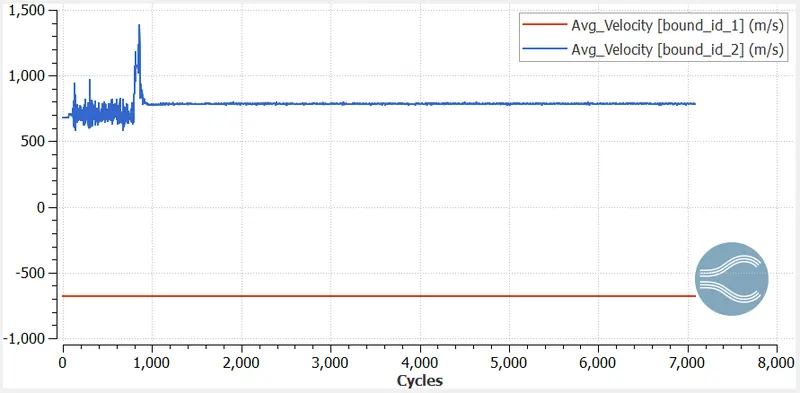
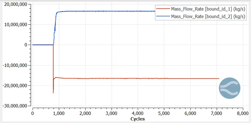
Mass flow rate:
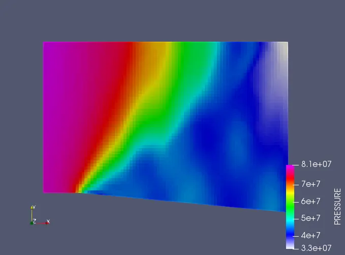
Pressure Contour:
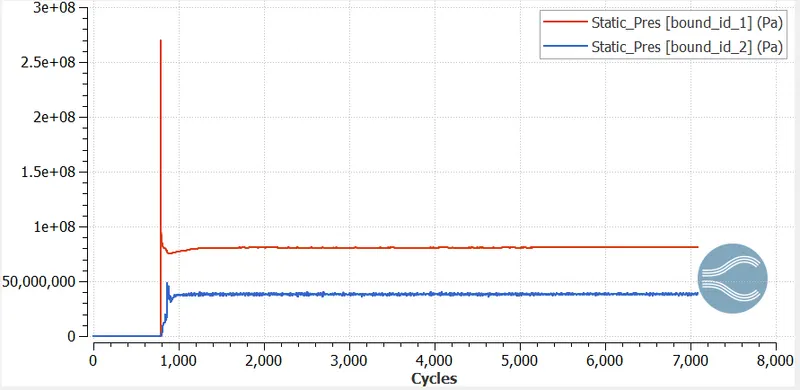
Pressure plot:
Temperature contour:
https://drive.google.com/file/d/1g4cwI6WZ5gRrWLfPXI_b2H9T3Y5K4EG7/view?usp=sharing
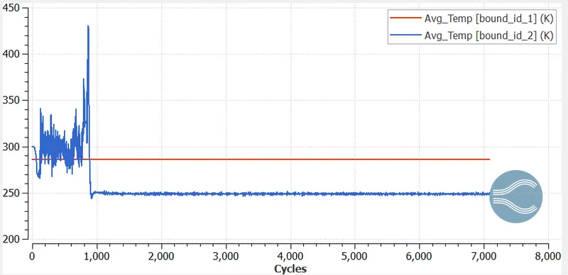
Temperature plot:
Mach number:
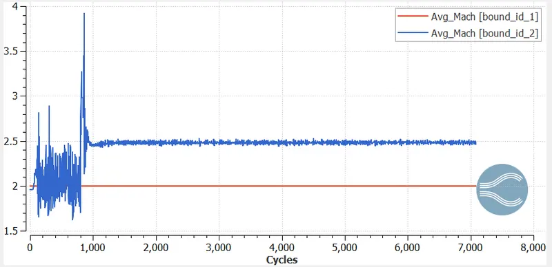
Case-2 : (Velocity = 690m/s, SGS = 0.03)
Velocity contour:
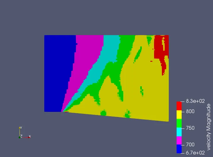
Velocity plot:
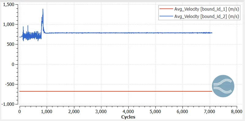
Mass flow rate:
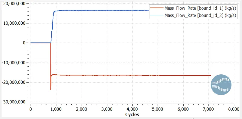
Pressure contour:
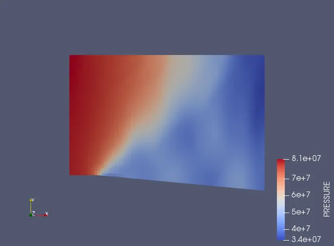
Pressure plot:
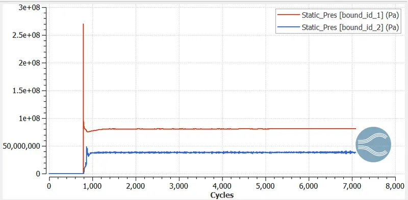
Temperature contour:
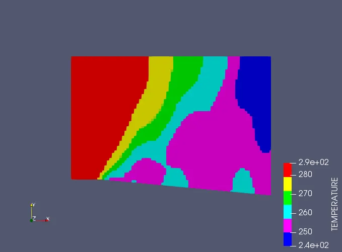
https://drive.google.com/file/d/1WqbshXrx55D7JHBOLL8MX6sECE6CrCVE/view?usp=sharing
Temperature plot:
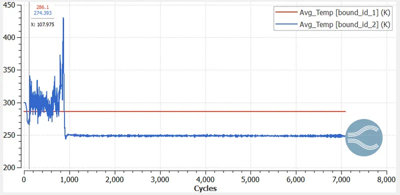
Case-3 : Velocity = 680m/s, SGS = 0.1
Velocity contour:
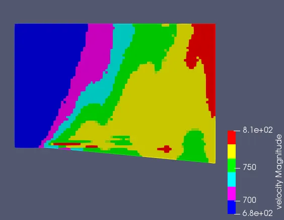
Velocity plot:
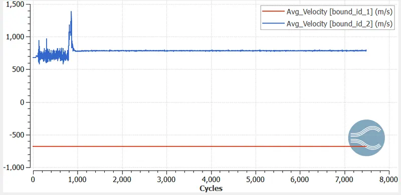
Mass flow rate:
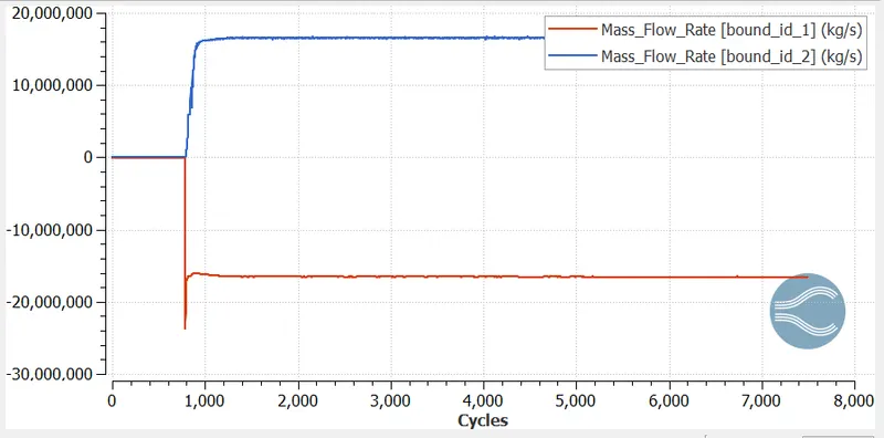
Pressure contour:
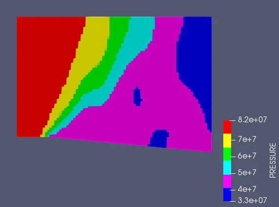
Pressure plot:
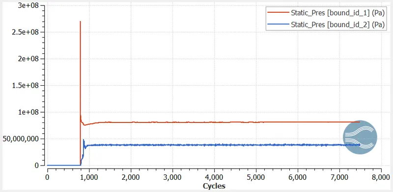
Temperature contour:
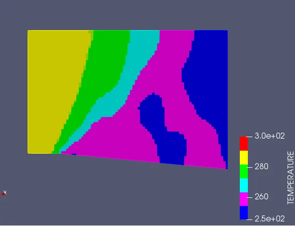
https://drive.google.com/file/d/1HnvcfFB6x9TAoDJQQPUt3Zptni_8JI-_/view?usp=sharing
Temperature plot:
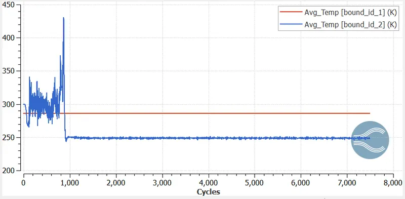
Mach number:
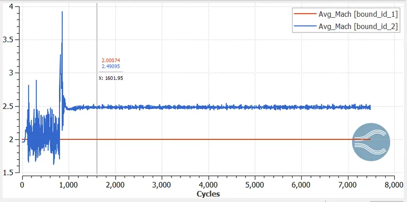
Observations:
- Increase in SGS decreases the cell count which means lower number of SGS value makes AMR more refine which causes increase in number of cells.
- Changing the SGS value from 0.05 to 0.01 and for 0.1, more level of details were captured.