Week 5: Prandtl Meyer Shock problem
AIM:
To simulate the Prandtl Meyer Shock flow in converge CFD
OBJECTIVE:
1.To explain Shock flow boundary conditions
To do a literature search on what BC's are typically used for shock flow problems
2.To describe what is Shock wave and physics behind it
3.Effect of SGS parameter on Shock location and to look for the effect of SGS temperature value on cell count and shock location.
DESCRIPTION:
SHOCK WAVE:
Shock wave is a type of propagating disturbance that moves faster than the speed of sound in that medium. It carries energy and can propagate through a medium similar to an ordinary wave. But in the shock wave, there is an abrupt change in pressure, temperature and density of the medium.
It is a strong pressure wave in any medium air or water. It is created by supersonic aircraft, explosions, linghtning or other phenomenon that creates violent changes in pressure. Their speed increases as the amplitude is raised. The amplitude of strong shock wave, as created in the air by an explosion, decreases almost as the inverse square of the distance until the wave has become so weak that it obeys the laws of acoustic waves.
PRANDTL-MEYER EXPANSION FAN:
A Prandtl-Meyer expansion fan also known as a supersonic expansion fan which is a centered expansion process that occurs when a supersonic flow turns around a sharp corner or a convex corner. It consists of infinite Mach waves diverging from the sharp corner. Each wave turns the supersonic flow in small steps. A supersonic flow cannot turn through a single shock wave because that would violate the second law of thermodynamics.
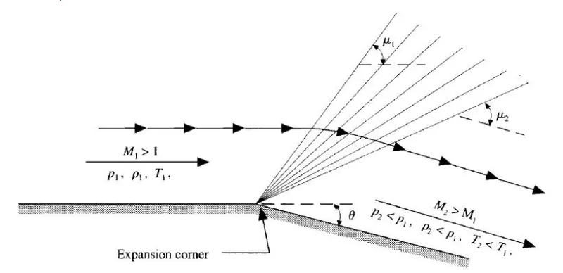
The above image shows the expansion fan ( a set of diverging lines from the corner). As the flow passes through the expanision fan the velocity increases and thereby the Mach number increases while the static pressure, temperature, and density decreases. This process if isentropic and that is why the stagnation properties ( the total pressure and total temperature) remain constant across the fan.
SHOCK FLOW BOUNDARY CONDITIONS:
1.Dirichlet Boundary condition
In the dirichlet BC, the value of the function is specified at the boundary y=f.
2.Neumann Boundary condition
In the Neumann BC, the value of the normal derivative of a function is specified.
`(dely)/(deln)=f`
3.Robin Boundary condition
It is the combination of both the above BCs, specified at both ends `c0.y+c1.((dely)/(deln))=f`
4.Mixed Boundary conditions
On one end there is a Dirichlet BC and on the other end there is a Robin BC.
WHY THE NEUMANN BOUNDARY CONDITION IS USED FOR SUPERSONIC OUTLETS
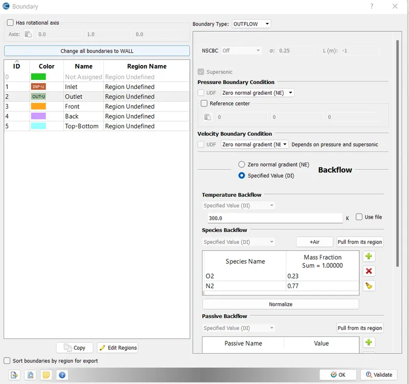
Because the values of all the variables (pressure, velocity, temperature, Mach no) are not available before solving the problem, so nothing is specified at a supersonic outlet and all variables are extrapolated from the domanin interior. Only the Normal derivative (normal w.r.t the outlet boundary) of variables are specified as 0 i.e zero gradient.
However, if any pressure value or velocity is specified at the outlet the solution will not converge and becomes unstable.
STEPS USED FOR SETTING UP THE SIMULATION:
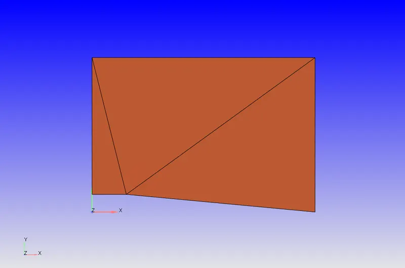
Opening the geometry in Converge studio as follows
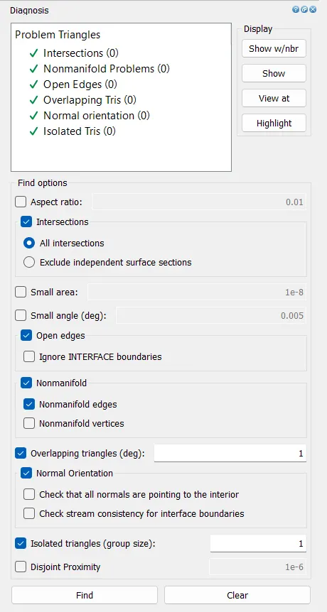
Running the diagnosis we see no errors
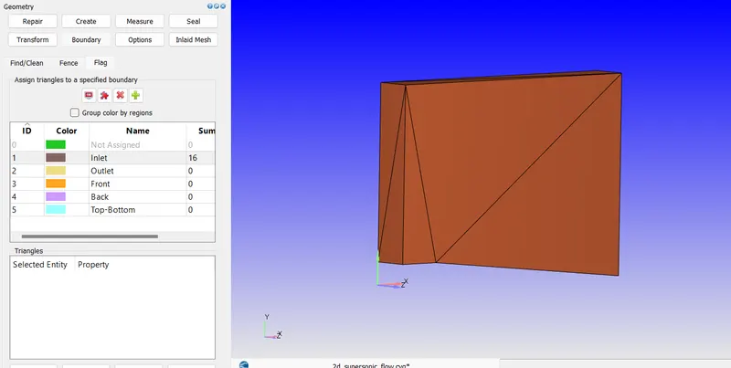
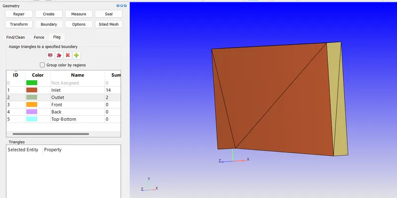
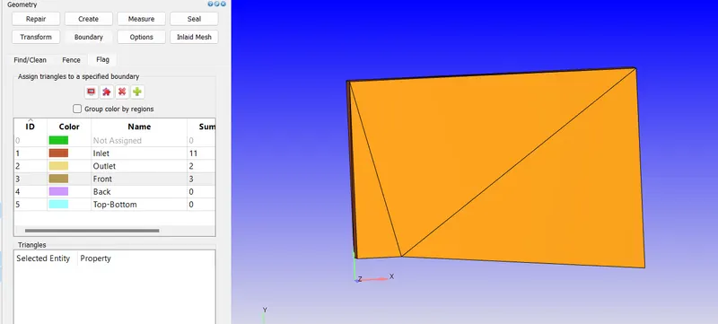
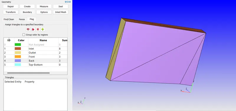
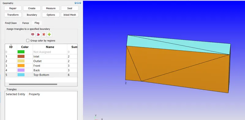
Now flagging the boundaries as follows
For inlet
For outlet
For front
For back
For Top and bottom
Now checking for Normals to point inwards
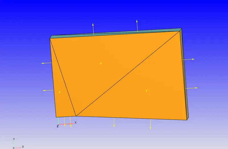
As they are pointing outwards and fluid flows inside, we need to transform them to inwards as follows
Hiding the front face we see normals inside
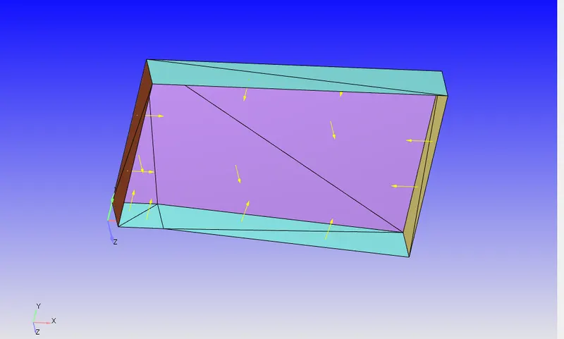
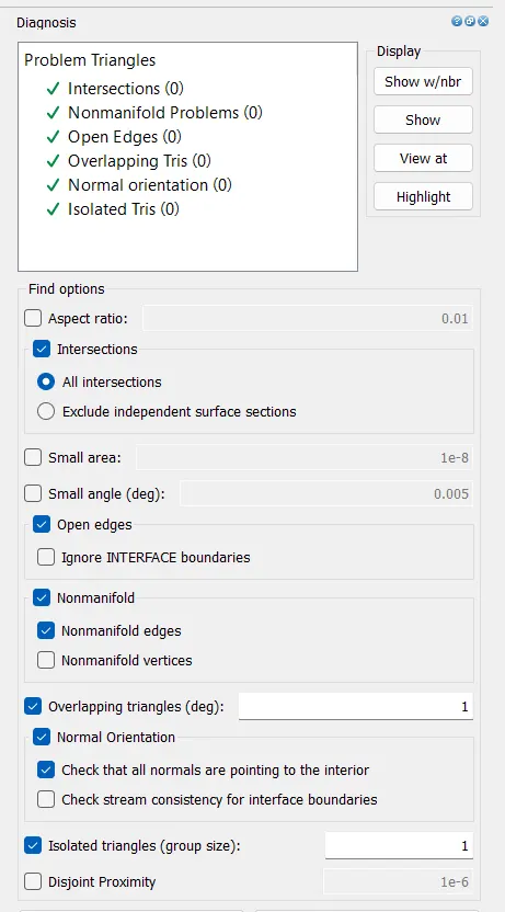
Again checking for diagnosis with normals checked inside as follows, we see no errors
Now setting up the case
In this simulation we run the case for 4 set-ups as follows
Case-1: with velocity 680 m/s (Supersonic flow) and SGS parameter 0.05
Case-2: with velocity 680 m/s (Supersonic flow) and SGS parameter 0.01
Case-3: with velocity 680 m/s (Supersonic flow) and SGS parameter 0.9
Case-4: with velocity 100 m/s (Subsonic flow) and SGS parameter 0.05
We use Time based case-set up
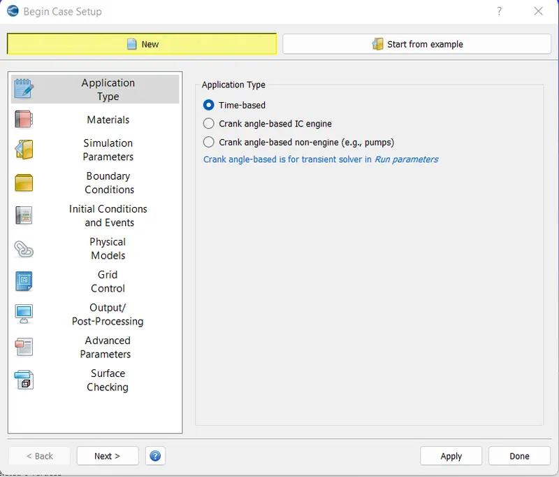
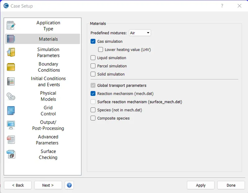
With materials as air
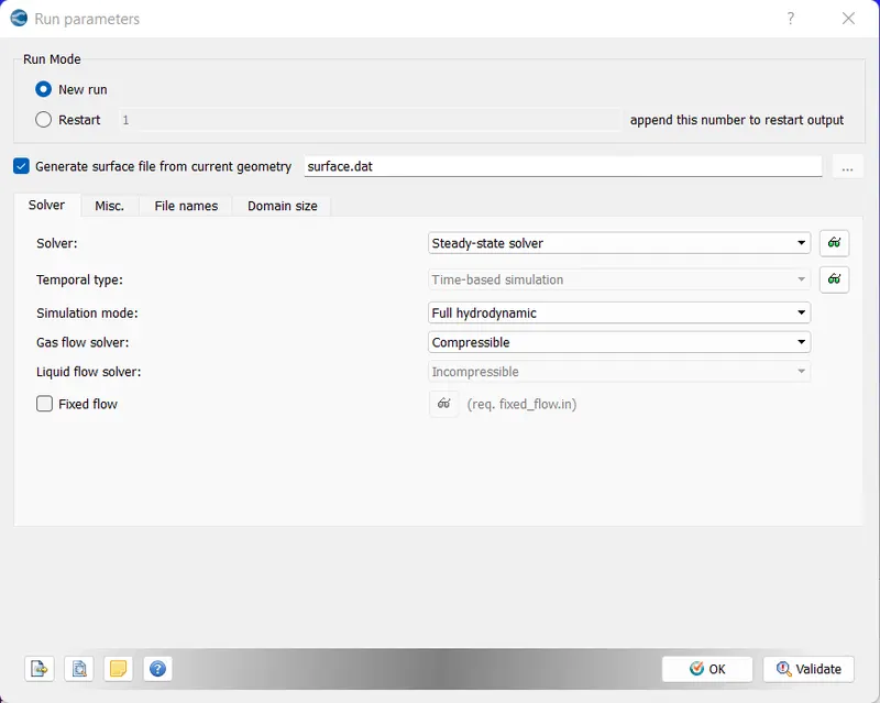
Run parameters, as steady state solver with full hydrodynamic compressible
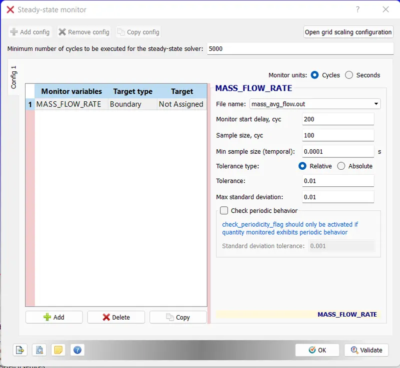
Steady state monitor as
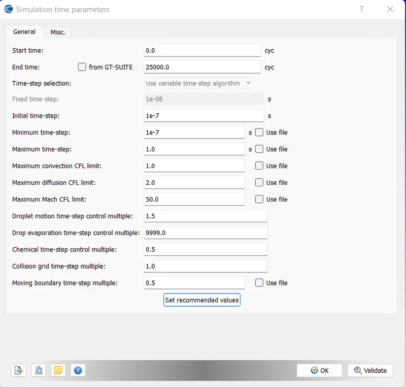
For Run time parameters
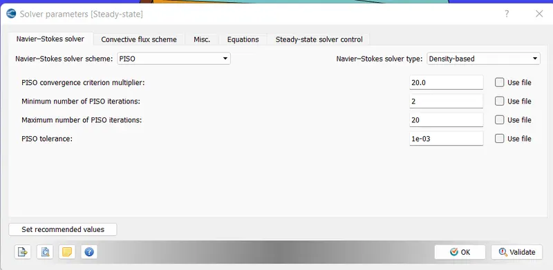
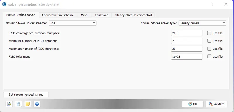
Solver parameters, Navier strokes with density based PISO solver and CFL limit 0.5
Boundary conditions are
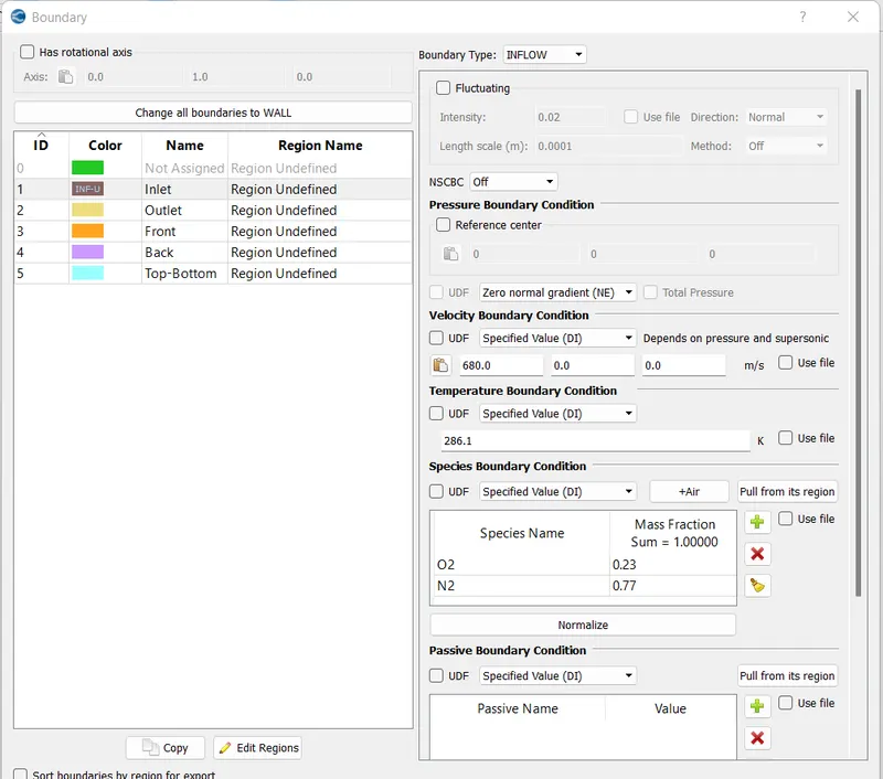
For inlet, with inflow and velocity along x-axis 680m/s supersonic velocity and temperature 286.1K. We know that at 286K speed of sound is 340, so inlet Mack number is 2.0
And for outlet boundary, we set it to Neumann-boundary conditions with Air flow as follows
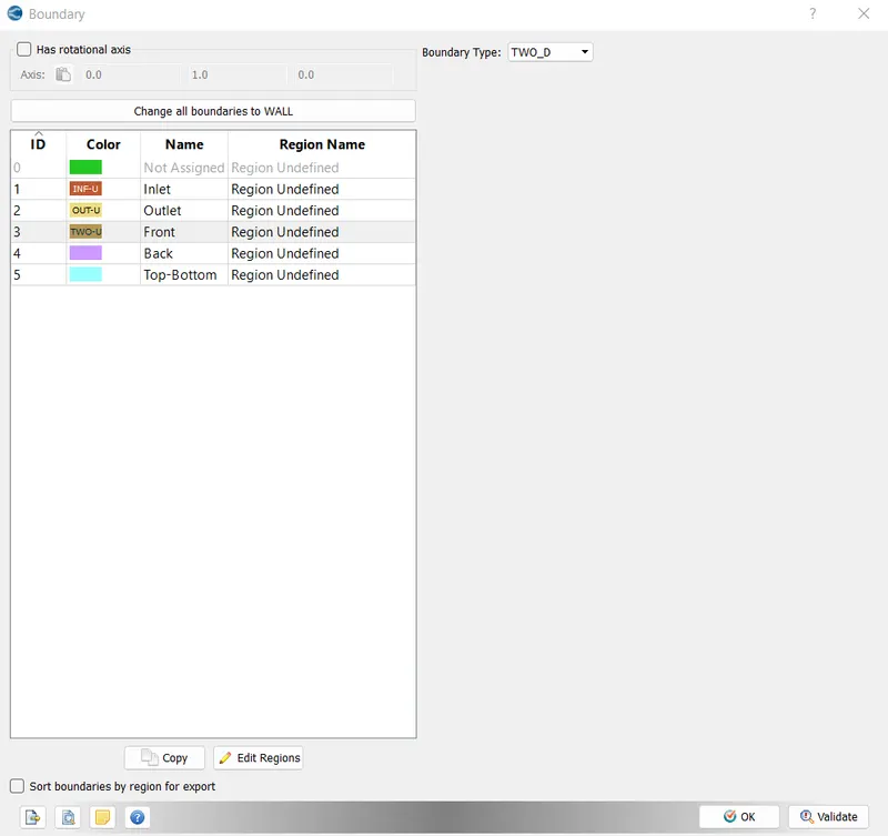
Front and back as Two-D as there is now floe in Z-direction
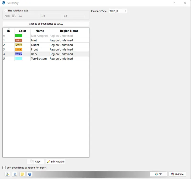
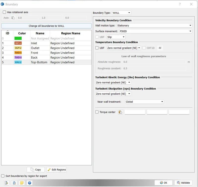
For Top-bottom boundary as slip
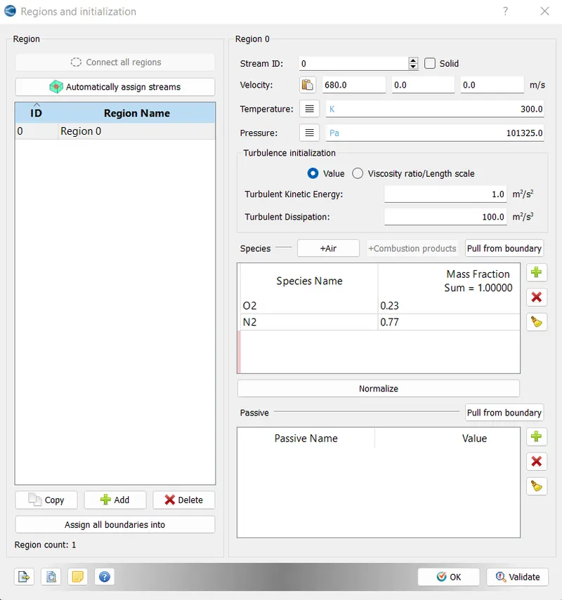
Initialization Regions for super-sonic with 680 m/s and for sub-sonic with 100m/s
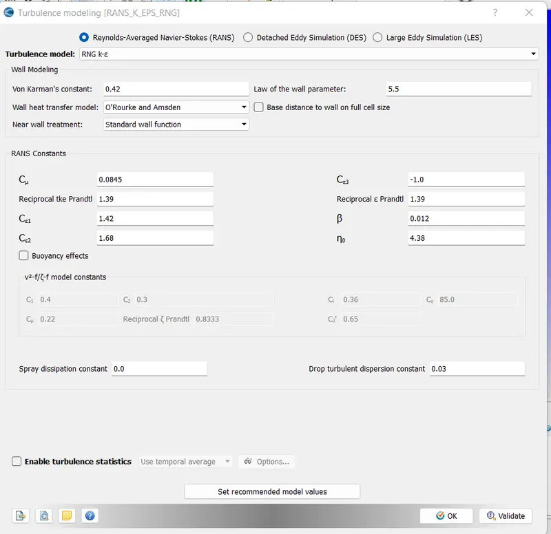
For turbulence model we use RNG k-epsilon with default values
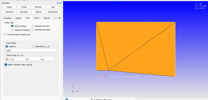
Scaling the dimensions with factor of 0.001 to meters
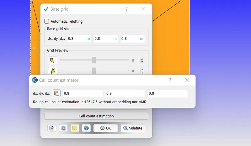
Base grid sizing as follows with 0.8 m
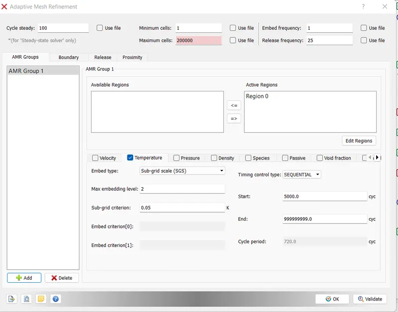
And then enabling the adaptive mesh refinement as follows
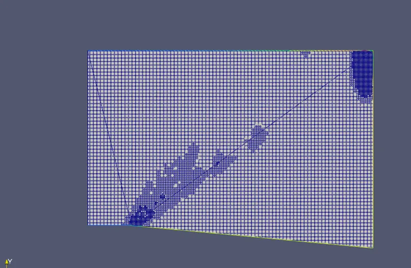
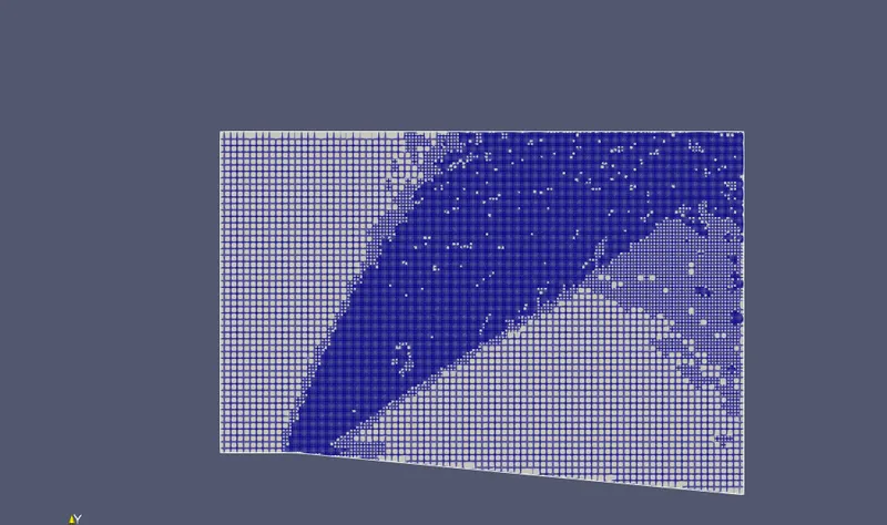
Adaptive mesh refinement is used so that the place where the shock occurs there the mesh to be finer to adapt the results in better way.
We know that, Grid size = `(Base grid)/(2^(n))`
n = embed level
And here Base grid is 0.8m and embed-level(n) is 2 Grid size=`(0.8)/(2^2)`= 0.2m is the smallest cell we will have in AMR
For case-1 Supersonic
For Case-2 SGS is 0.01 Super-sonic
For Case-3 SGS is 0.9 Super-sonic
For Case-4 SGS is 0.05 Sub-sonic
Now for post-processing output files
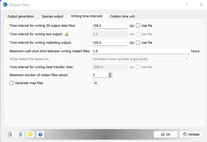
Then running the case set-up after exporting the input files to the folder using Cygwin.
By using the application mpiexec.exe & converge.exe by command line 'mpiexec.exe -n 2 converge.exe restricted' we run the simulation till results are converged.
Then using converge and paraview post processing results are observed and studied.
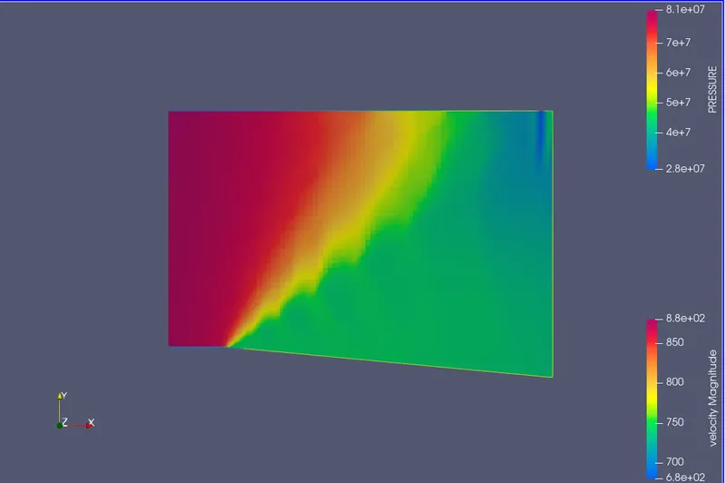
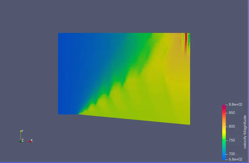
CASE-1: FOR SUPERSONIC WITH 680m/s AND SUB-GRID SCALE 0.05K
With Mesh size of dx=dy=dz = 0.8m
With Supersonic velocity in X-direction of 680 m/s
With Region initializaion of 680m/s in X-direction
With Adaptive Mesh refinement of SGS 0.05
The Mesh looks as follows
The Pressure Contour is
The velocity contour is
Animation for Velocity contour is
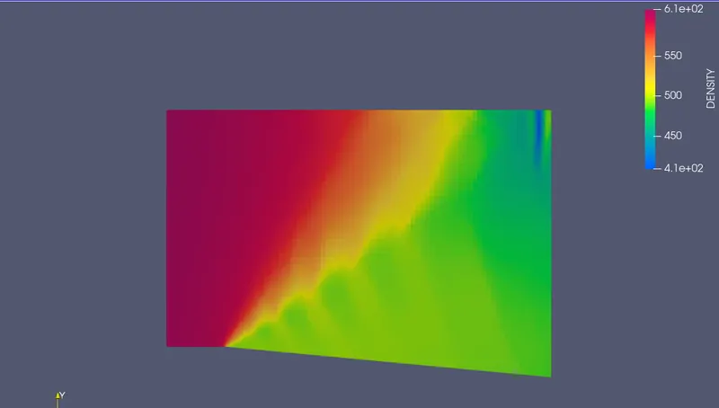
The Density contour is
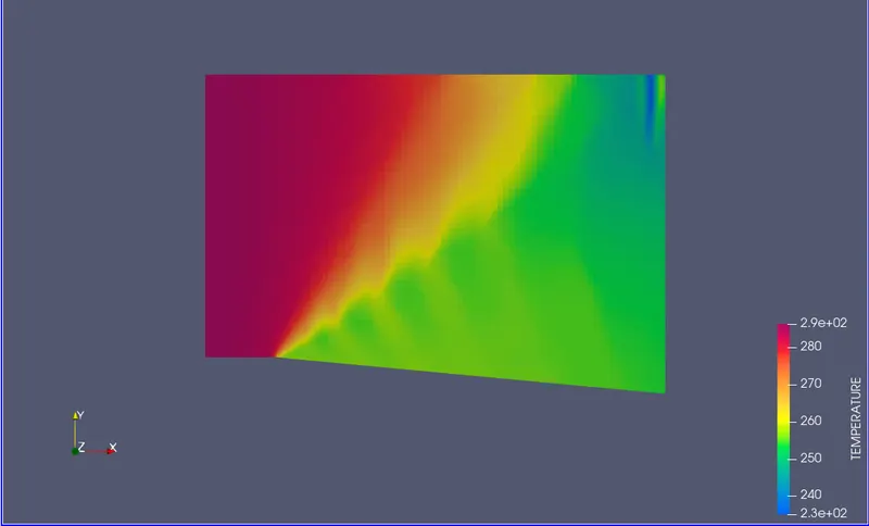
The Temperature contour is
Animation for temperature contour is
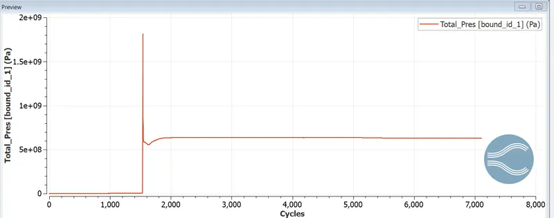
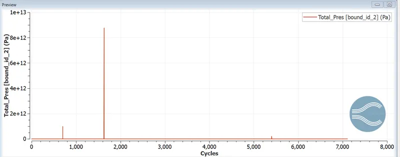
The Total pressure plots is
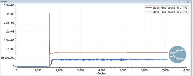
The Static pressure plots is
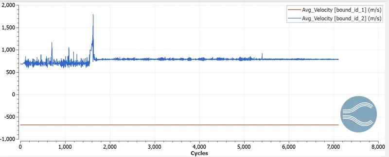
The Velocity plots is
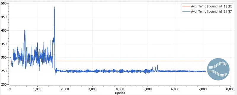
The Temperature plots is
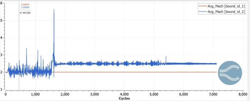
The Mach number plot is
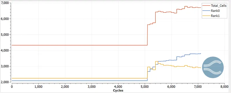
The Cell count plot is
CASE-2: FOR SUPERSONIC WITH 680m/s AND SUB-GRID SCALE 0.01K
With Mesh size of dx=dy=dz = 0.8m
With Supersonic velocity in X-direction of 680 m/s
With Region initializaion of 680m/s in X-direction
With Adaptive Mesh refinement of SGS 0.01K
The Mesh looks as follows
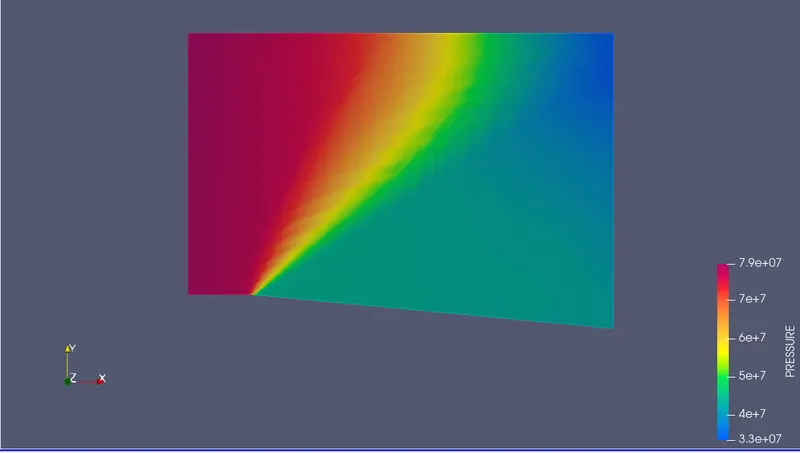
The Pressure Contour is
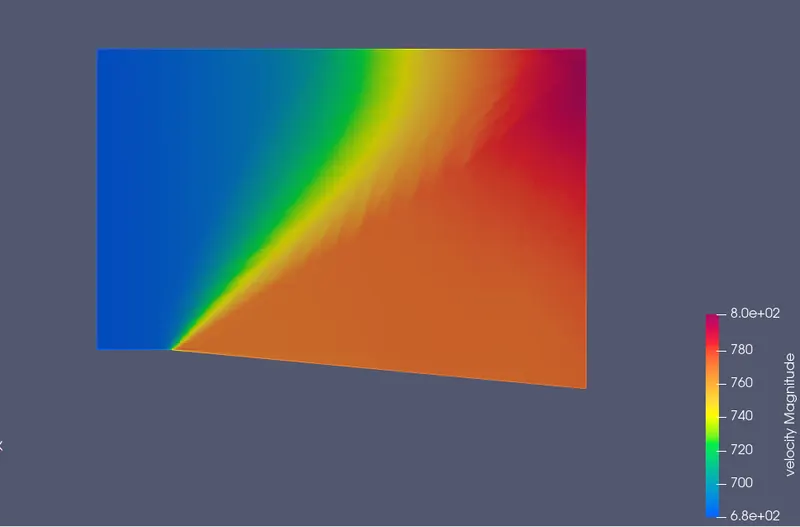
The velocity contour is
Animation for Velocity contour is
The Density contour is
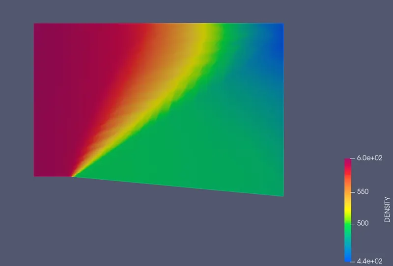
The Temperature contour is
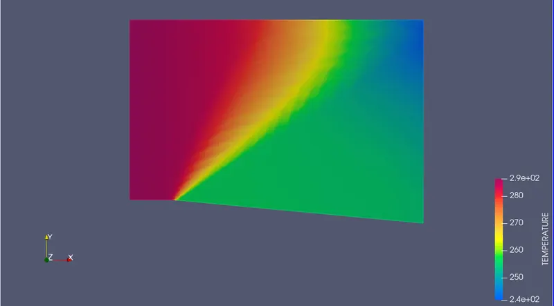
Animation for temperature contour is
The Total pressure plots is
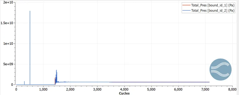
The Static pressure plots is
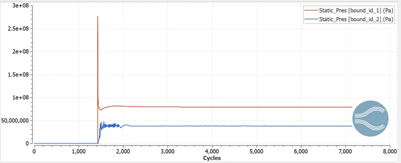
The Velocity plots is
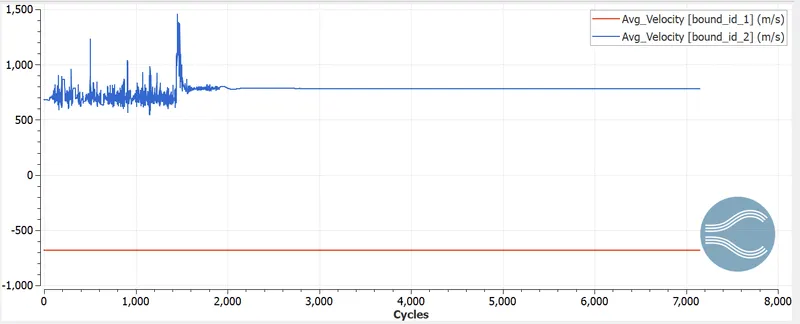
The Temperature plots is
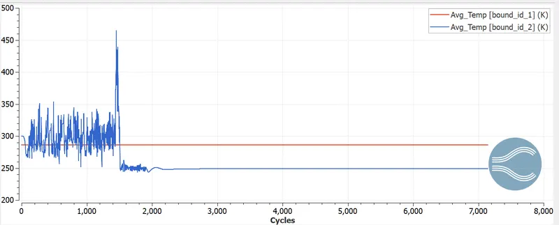
The Mach number plot is
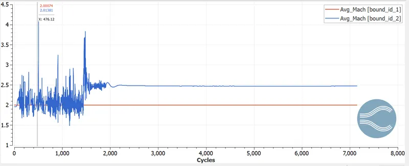
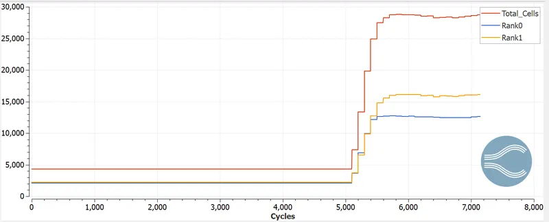
The Cell count plot is
CASE-3: FOR SUPERSONIC WITH 680m/s AND SUB-GRID SCALE 0.9K
With Mesh size of dx=dy=dz = 0.8m
With Supersonic velocity in X-direction of 680 m/s
With Region initializaion of 680m/s in X-direction
With Adaptive Mesh refinement of SGS 0.9K
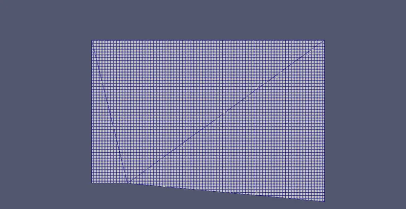
The Mesh looks as follows
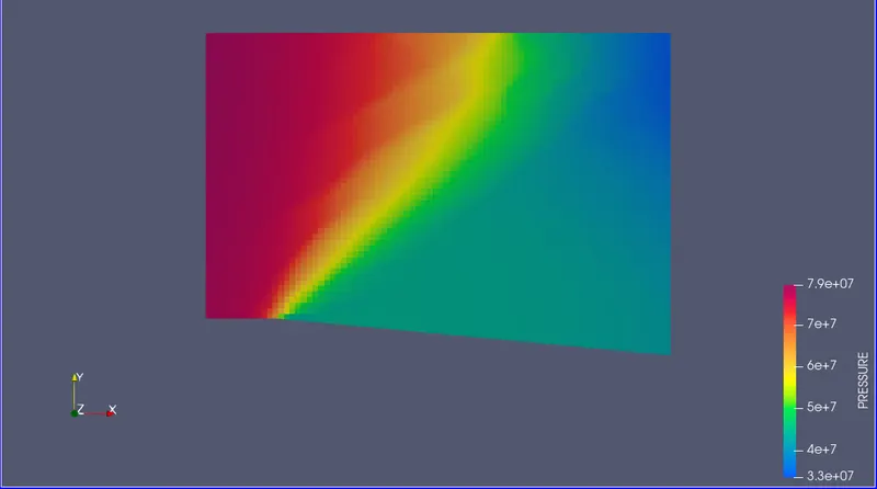
The Pressure Contour is
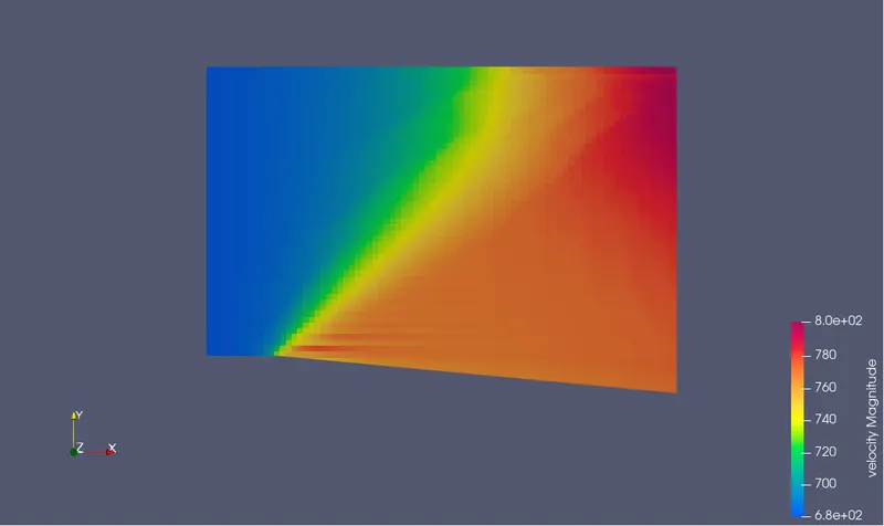
The velocity contour is
Animation for Velocity contour is
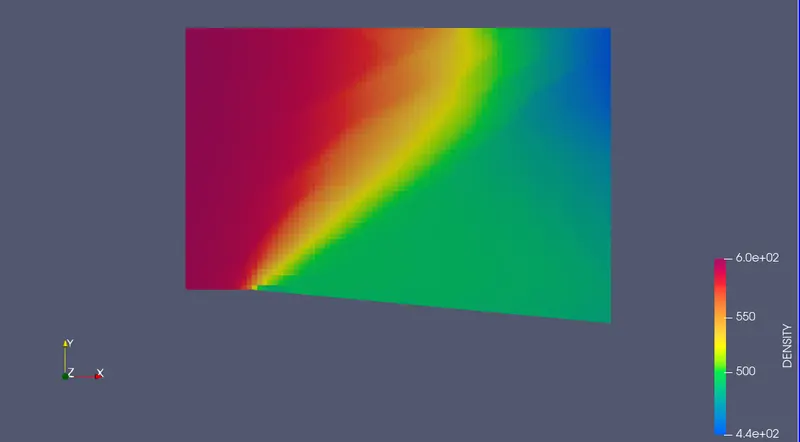
The Density contour is
The Temperature contour is
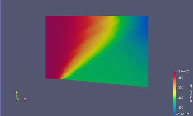
Animation for temperature contour is
The Total pressure plots is
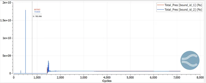
The Static pressure plots is
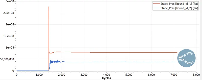
The Velocity plots is
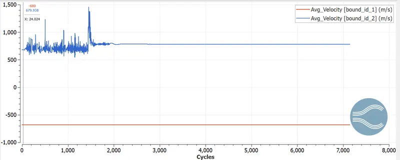
The Temperature plots is
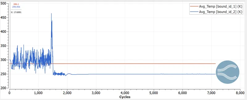
The Mach number plot is
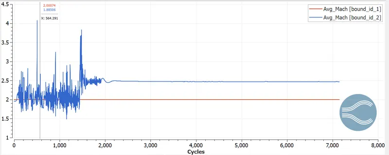
The Cell count plot is
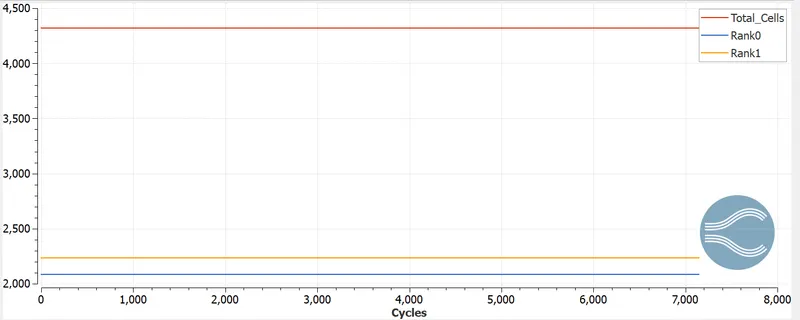
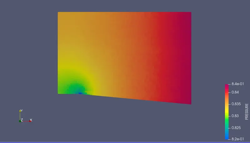
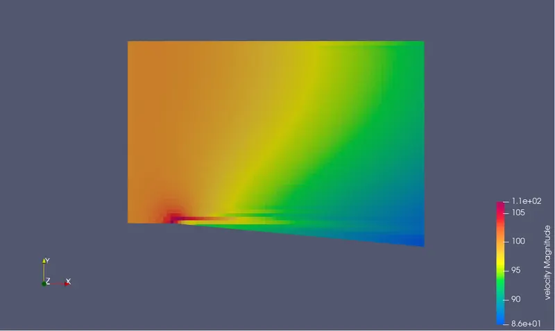
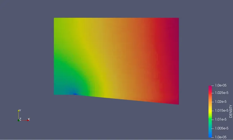
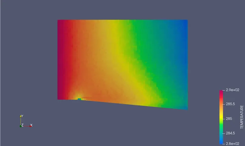
CASE-4: FOR SUB SONIC WITH 100m/s AND SUB-GRID SCALE 0.05K
With Mesh size of dx=dy=dz = 0.8m
With Sub Sonic velocity in X-direction of 100 m/s
With Region initializaion of 100m/s in X-direction
With Adaptive Mesh refinement of SGS 0.05
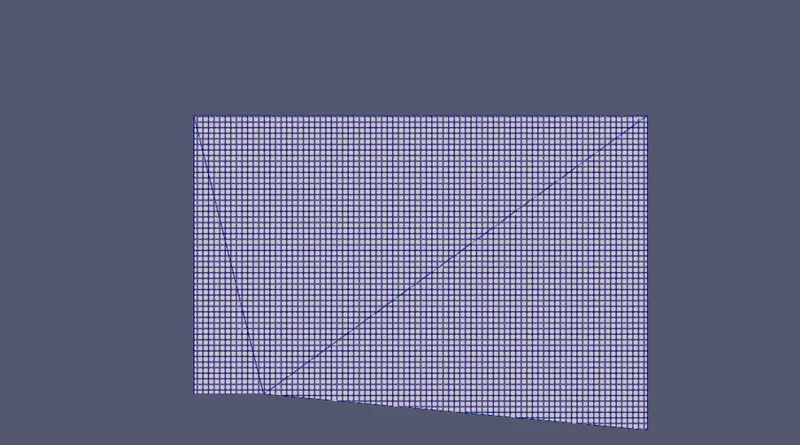
The Mesh looks as follows
The Pressure Contour is
The velocity contour is
Animation for Velocity contour is
The Density contour is
The Temperature contour is
Animation for temperature contour is
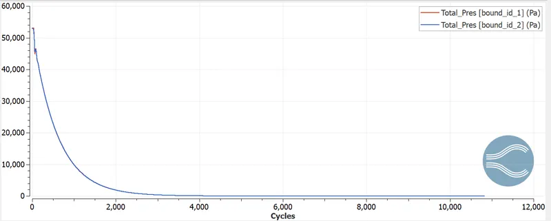
The Total pressure plots is
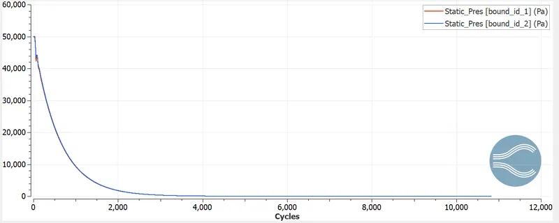
The Static pressure plots is
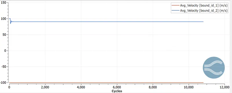
The Velocity plots is
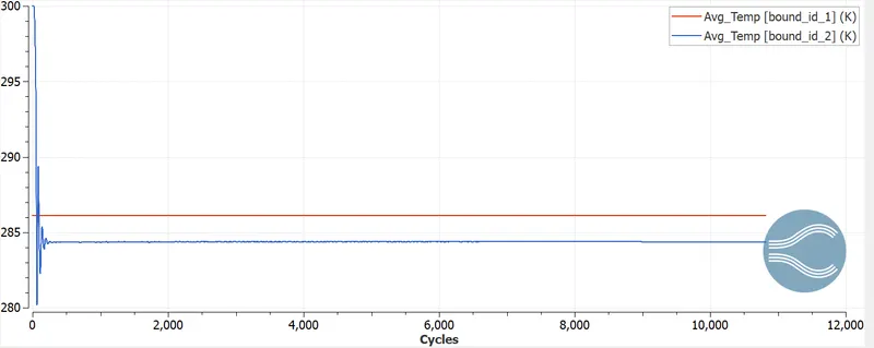
The Temperature plots is
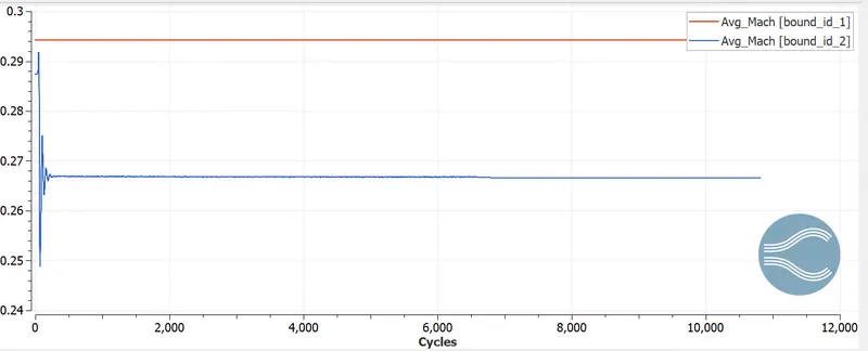
The Mach number plot is
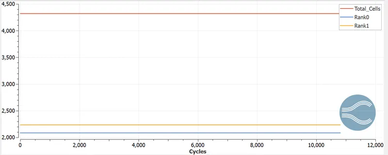
The Cell count plot is
EFFECT OF SGS ON TOTAL CELL COUNT:
From the above all plots we can clearly observe that as the SGS value decreases then the refinement of cells takes place thus it indicates the increase in the cell count.
For the low SGS value the number of cells is more due to higher refinement, thus higher refinement means higher number of cells.
SUB SONIC Vs SUPER SONIC FLOW COMPARISION
In supersonic flow, the prandtl-mayer expansion fan is clearly visible and the mesh refinement is also visible in the shock region.
Whereas on the other hand, in the case of subsonic flow, the prandtl meyer expansion fan is not at all visible and even the mesh refinement is not visible. This is because there are no sudden fluctuations in pressure, velocity, temperature or density or in other words shocks.
Also, the average Mach number increases from the inlet to the outlet in case of supersonic flow and decreases in case of subsonic flow.
CONCLUSION:
From the post processing results, it is observed that the expansion fan tends to becoms wider and distinct as the SGS parameter increases.
A higher value of SGS will limit the mesh refinement required to capture the expansion waves effectively leading to wide, blurry and improperly refined waves.
From the comparision plot of the SGS parameter, it is seen that a lower number of SGS parameters gives out higher refinement which in turn will have higher number of cells.