Week 5: Prandtl Meyer Shock problem

Aim- Prandtl Meyer Shock problem

Introduction –

Shock flow boundary conditions-

Boundary value is differential equation with set of constraint is known as boundary condition. The solution to boundary value is solution to the differential equation which also satisfy the boundary equation as well.

Types of Boundary condition –

Dirichlet boundary condition –

In this boundary condition when imposed on partial differential equation, it specifies the value that a solution need to on along the boundary of the domain.

Neumann boundary condition –

In this boundary condition when imposed on partial differential equation, it specifies the value in which the derivate of solution is applied within boundary of domain.

Robin boundary condition –

In this boundary condition when imposed on partial differential equation, it is specification of a linear combination of value of a function and the value of its derivation on boundary of the domain.

Mixed boundary condition –

In this boundary value problem in which the solution of given equation is required to satisfy different boundary condition on disjoint part of boundary of the domain where the condition is stated.

What is a shock wave –

Shock wave in medium such as air, water, or a solid substance, produced by supersonic phenomena that create violent changes in pressure. In shock wave the pressure and temperature changes abruptly. Its speed inc as amplitude is increases.

Steps –

1. Geometry
2. Define the boundary
3. Case setup
4. Simulation
5. Post processing
6. Outputs
7. Conclusion

Geometry –

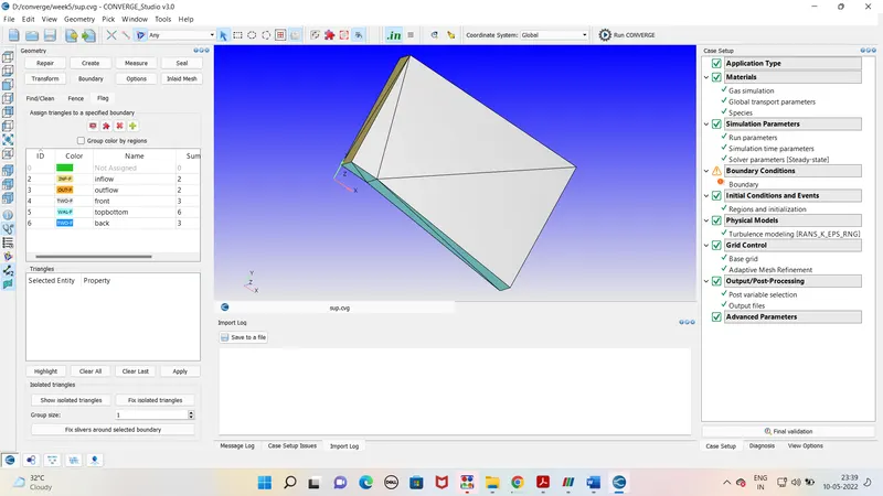
Import the geometry in converge .

Do boundary flagging as inlet , outlet , 2d and walls. Run the diagnosis and check for any error.

Case setup –

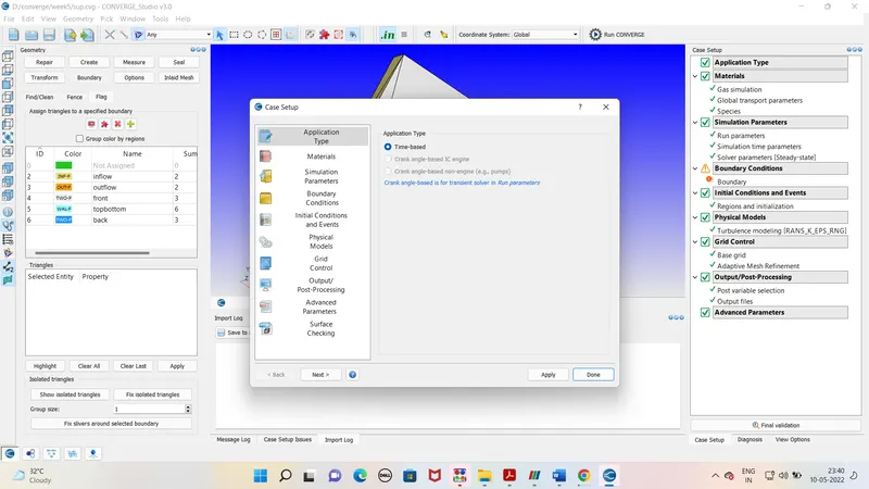
Application type –

Pre defined mixture -

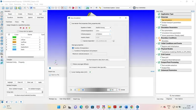
Gas simulation –

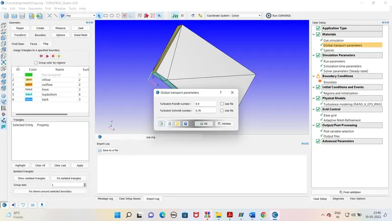
Global transport parameter –

species –

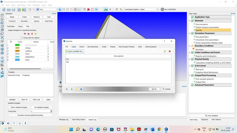
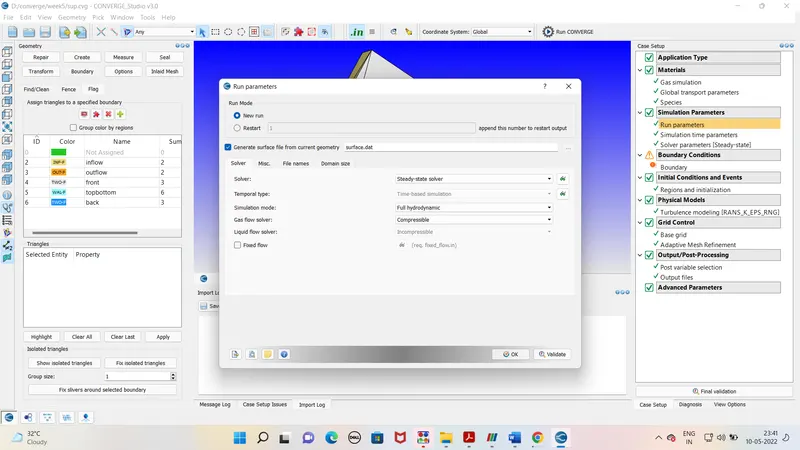
Simulation Parameter –

Run parameter –

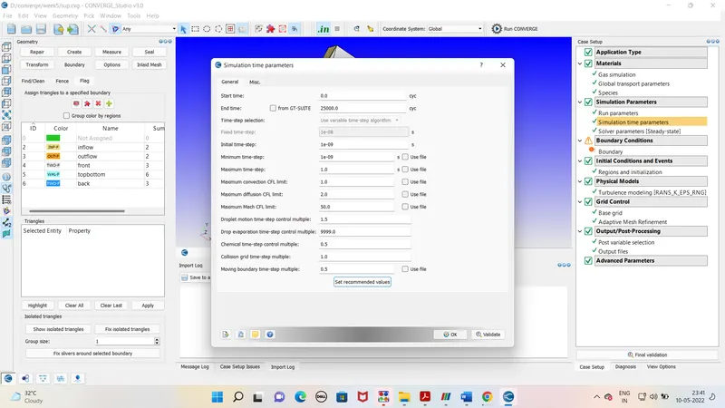
Simulation time parameters-

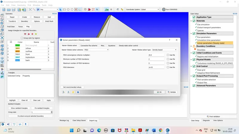
Solver parameters-

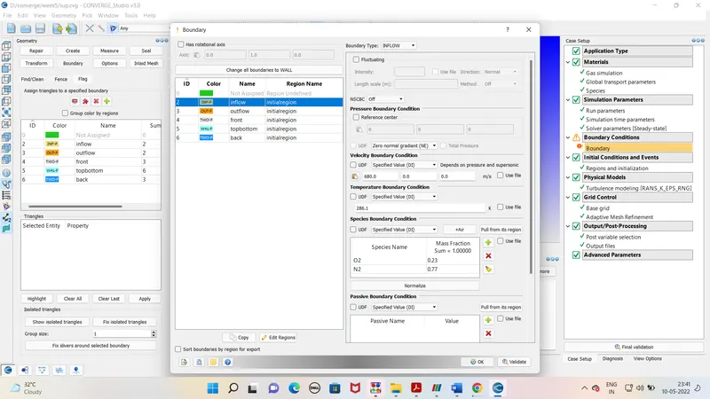
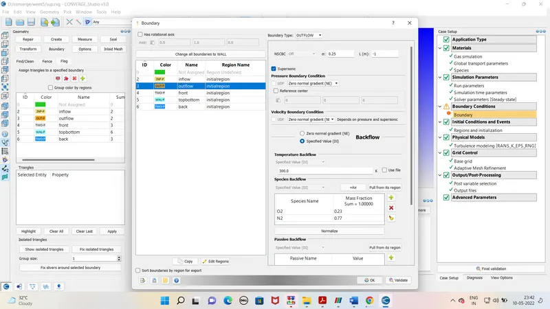
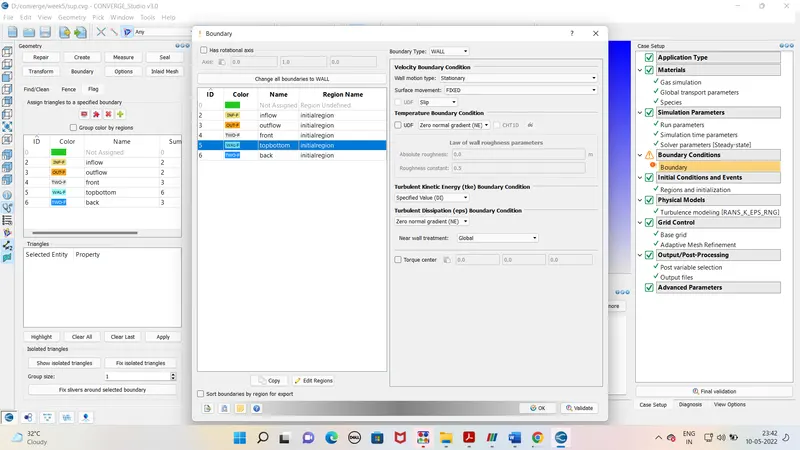
Boundary condition –

Inlet

Outlet

Define Front and back side as 2D boundary type –

Top and bottom wall –

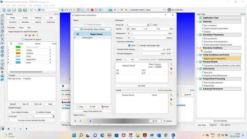
Intial condition and events –

Physical models –

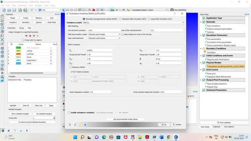
Grid control –

Base grid – dx - 0.8 dy –0.8 dz – 0.8

Adaptive mesh refinement

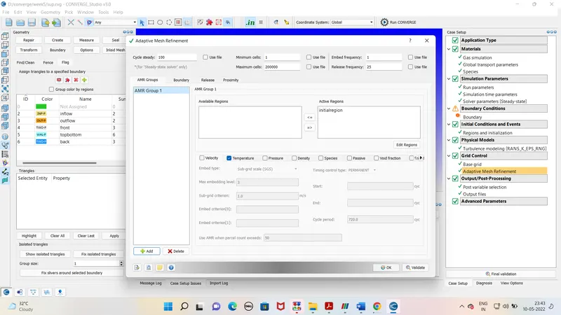
Output processing Advanced parameter – Default

After case set up exports the file to defined folder. Run the simulation in the Cygwin. Generate the output files. As output file is generated run the post processing in Cygwin again. Open the output file in paraview for the mesh view and contours. For excessing pressure , velocity and mass flow rate use line plotting tab.

Outputs –

Mesh

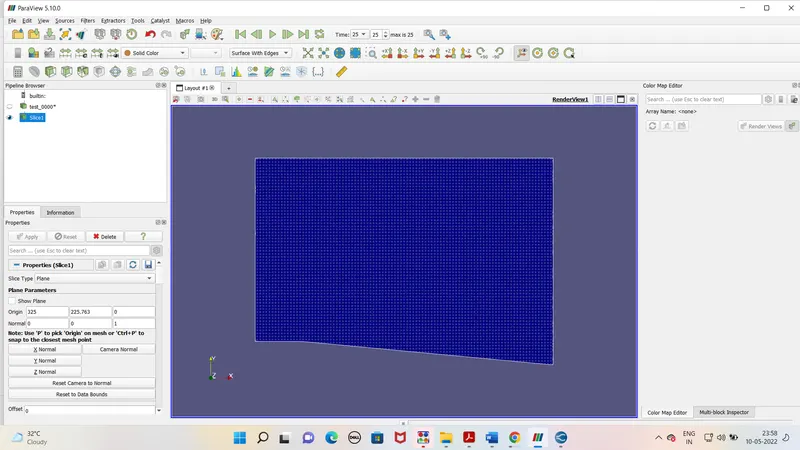
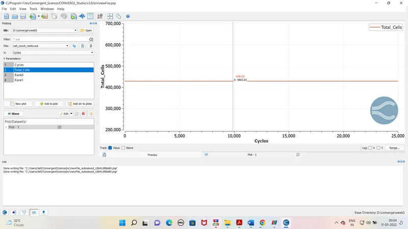
Total cell -

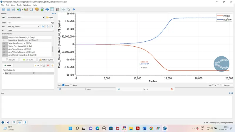
Mass flow rate at inlet and outlet.

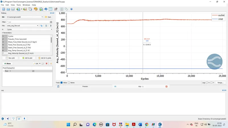
Avg velocity

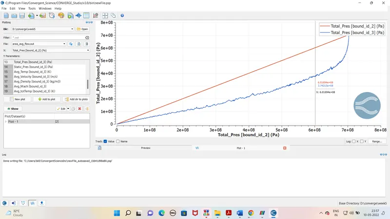
Total pressure

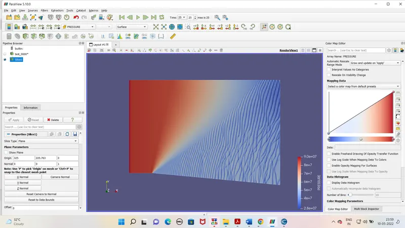
Pressure contour

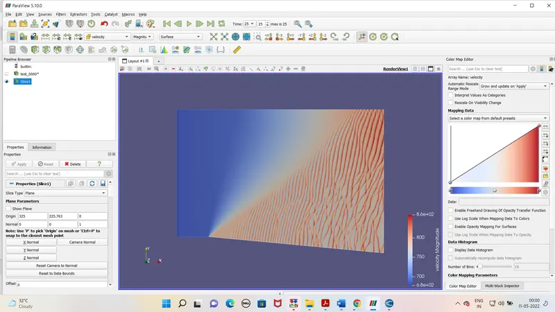
Velocity contour

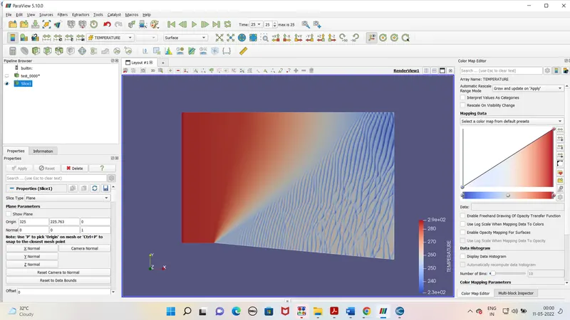
Temprature contour

Animation links -

https://youtu.be/sLyl_kd8-fQ

https://youtu.be/sLyl_kd8-fQ

Conclusion -

Animation of output results is shown above .It is seen prandtl meyer expansion is clearly visible.Shock region is also visible.

The plots at inlet and outlet are shown above.