Week 5: Prandtl Meyer Shock problem
Aim: Simulate Prandtl Meyer Shock Problem using converge and post process the results using paraview.
SHOCK WAVE:
Shock waves gets generated when a object moves faster than the speed of sound(supersonic speed), moreover there is an abrupt change in the flow area or diversion, the flow process remains irreversible and the entropy rises.
Shock waves are very small regions in the gas where the gas properties changes by large amounts. Across a shock wave, the static pressure, temperature and gas density rises instantaneously.
Shocks can be of three types:
Normal Shock:
This can occur when shock is 90°(perpendicular) to the shock medium's flow direction.
Oblique Shocks:
This can occur when shock is at a certain angle to the shock medium's flow direction.
Bow Shocks:
This can occur upstream of the front of a blunt object when the upstream flow velocity exceeds Mach 1.
Boundary conditions in shock flows:
Neumann boundary conditions are used at the outlet in case of Shock flow problems. The outer boundary has no influence on the inner nodes, the values at the outlet is extrapolated from the inner nodes in Neumann boundary conditions. These boundary conditions include derivative of the solution at the boundary.
Dirichlet boundary condition is provided at the inlet. Dirichlet boundary condition provides the values that a solution needs to take along the domain boundary.
Prandtl Meyer Shock problem
When a supersonic flow encounters a convex corner, it forms an expansion fan, which consists of an infinite number of expansion waves centered at the corner.
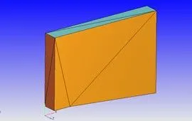
Geometry-
Inlet, Outlet, 2D front, 2D back and top and bottom slip boundary given.
Setup-
Applications-
Time-Based
Materials used:
Species-Air (O2, N2)
Simulation Parameters:
- Run Parameter: Steady-state solver | Full Hydro. | Compressible
-Start time-0.
End time-15000 cycle
-Intial time step=minimum time step=1e-8 s
-Maximum time step=1 s
Max CFL limit(Convection/Diffusion): 1.0/2.0
Boundary conditions-
-Inlet- INFLOW-velocity-678m/s, Pressure - 101000 Pa, 286K, Air(Species)
-Outlet- OUTFLOW-pressure & velocity-Zero normal gradient
-Top & bottom- Wall- stationary, fixed, slip, 300k, Zero Normal Gradient for Turbulent kinetic energy boundary condition
-Front- 2D
-Back - 2D
Regions & Initialization:
Velocity and pressure set to 678 m/s and 50000 pa
Temp: 300K
Turbulence Initialization
Species- Air(O2,N2)
Turbulence Model:
No Turbulence model used.
Base grid- dx=dy=dz=0.8 m
Adaptive mesh refinement-SGC value-,0.5,1.0.
For sub grid criterion as 1.0:
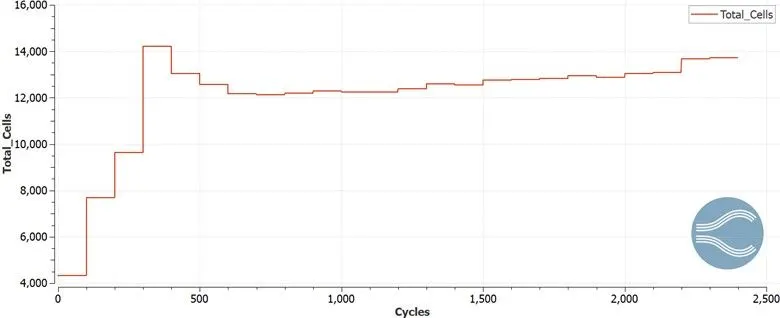
The total cells are shown below for the geometry and reaches close to 14000 for this simulation.
 :
:
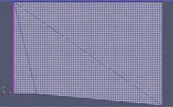
Mesh
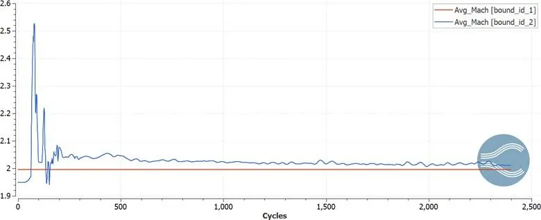
The graphs below show the effect of supersonic flow across mach no, pressure, temperature and velocity across the expansion wave.
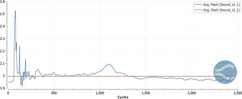
The mach no. graph shows the mach no at inlet and outlet. It shows the mach no reaches about 2.02 at the outlet and 2 at the inlet.
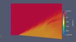
The Velocity contour below shows the change in velocity value across the expansion wave where, V1>V2.
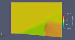
The temperature contour below shows the temperature difference across the expansion wave where T1>T2 across the distance.
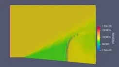
The pressure contour below shows the pressure difference across the expansion wave where the P1>P2 area.
For sub grid criterion 0.05:
Mesh
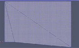
The total cells graph shows the total no of cells in geometry which is close to 20000.
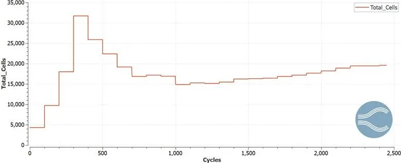
The graphs below show the effect of supersonic flow across mach no, pressure, temperature and velocity across the expansion wave with the sub grid criterion at 0.5.
The mach no graph shows the difference in mach across the inlet and outlet through the simulation. The mach no remains at 2.0 for the inlet while the value for outlet remains high initially and lesser as the cycles increase.
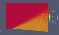
The velocity contour below shows the difference in the velocity across the expansion wave where the v1 is greater than v2.
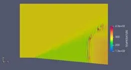
The temperature contour below shows the temperature variation as the expansion wave is reached where T1>T2.
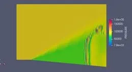
The Pressure contour shows the difference in pressure data through the supersonic flow, the pressure varies in the form P1>P2.
Conclusion:
The prandtl meyer shock problem was simulated using converge and post processed using paraview for different sgc values.
The sub grid criterion values were varied from 0.5 to 1.0 for the simulation.
The Mach no, velocity, temperature and pressure contour were analyzed.
The results were more accurate with lower sgc values.
Youtube Animation Link: