Week - 5 - Modelling Spotwelds

Skill-lync assignment 5

Aim: The objective of this assignment is to model spot welds for the given component, first as beam elements, and in a second iteration, as solid elements. The two iterations are then to be subjected to a crash simulation and the resultant stresses and strains are to be compared in order to establish the pros and cons of using either of these modelling approaches.

Case setup: The given component depicts a pair of crash tube sections that are meant to be joined together by a series of spot welds. The component is shown below.

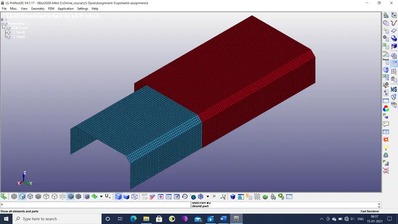
Figure 1: Crash tube assembly

As with the previous assignment, the crash tube is to have the following boundary conditions:s

1. Material: Steel (Elastic behavior)
2. Beam weld elements (1^st iteration), solid weld elements (2^nd iteration)
3. Initial velocity: 50 kmph or 13.8889 mm/ms

Output files: The following plots & output files are to be derived through post-processing: -

1. D3plot, glstat, sleout and rcforce output files.
2. Cross-sectional force in longitudinal direction.
3. Acceleration of a node in the middle of the crash tube.
4. Longitudinal stress and strain
5. Total, internal, kinetic, hourglass and sliding energies.
6. Tensile and shear stress & strain in one weld element.

Procedure: The component is pre-processed through the following series of steps: -

1. The component is imported into the LS-Dyna workspace.
2. A shell section with a thickness of 1.5 mm and element formulation type 16 (fully integrated shell element) is defined and assigned to the component.
3. Steel with piecewise linear plastic behavior is assigned to the part via the MAT>24_PIECEWISE_LINEAR_PLASTICITY keyword. Referring to literature, the following properties are assigned to the material.

• Density: 7.8 X 10-6 kg/mm³
• Young’s modulus: 210 kg/(mm*ms²)
• Poisson’s ratio: 0.33
• Yield strength: 0.4 kg/(mm*ms²)
• Tangent modulus: 0.25 kg/(mm*ms²)
• Plastic failure strain: 0.14

Stress-strain curve for the material is defined as the following graph.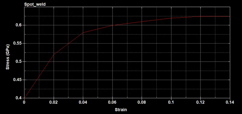

Figure 2: Stress-strain curve of steel

4. A node set is created for the nodes in the component via the create entity tool, in order to assign an initial velocity. The SET_NODE_LIST keyword is used for this purpose.
5. A rigid wall is created at the x-coordinate of 405 mm with a friction coefficient of 0.1. The node set defined earlier is set as the slave nodes of this rigid wall.
6. A part set is defined for the entire component, in order to define self-contact for it.
7. Self-contact is established within the crash tube via the CONTACT>AUTOMATIC_SINGLE_SURFACE keyword. The master set node ID is set as 0, signifying self-contact. The slave segment type (SSTYP) is set to 2 (part set ID).
8. An initial velocity of 13.8889 mm/ms is applied to the node set defined for the crash tube via the INITIAL>VELOCITY keyword.
9. The element editing tool is used to create 7 beam elements that represent spot welds, as shown below.

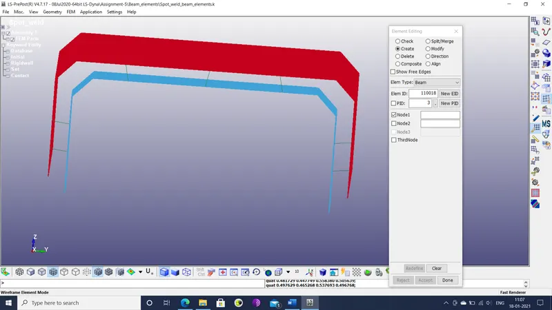
Figure 3: Spot weld beam elements

10. A new beam section is defined for the beam elements with an element formulation of 9 (spot weld beam) and a cylindrical profile with a beam thickness of 5 mm.
11. The MAT>100-SPOTWELD keyword is added to the spot weld part, in order to define its material. In addition to the material properties defined for the steel in the main component, a time of failure (TFAIL) of 1 ms is specified.
12. The CONTACT>TIED_SHELL_EDGE_TO_SURFACE keyword is edited to establish contact between component and beam elements.
13. The CONTROL>CONTACT keyword is edited so that initial penetrations (ISLCHK: 2) and thickness changes (THKCHG: 1) are considered.
14. The CONTROL>HOURGLASS and CONTROL>SHELL keywords are added to the file.
15. The CONTROL>TERMINATION keyword is edited so that minimum time step (DTMIN) is 0.0005 ms and run time (ENDTIM) is 2 ms.
16. The DATABASE>ASCII_option keyword is edited to include glstat, rcforc, sleout and swforc files as output. In addition, minimum time interval between plot points (DT) is set as 0.001 ms and binary output is set as 3 (output in ASCII file and in binary file).
17. A cross-section is defined by a set of nodes and shell elements in the location illustrated below.

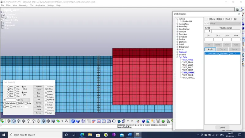
Figure 4: Shell element set for cross-section

18. The DATABASE>CROSS_SECTION_SET keyword is defined for this cross-section and the DATABASE>ASCII_option is edited to include the results at the cross-section in a secforc file.
19. The model checker is run to check the component for any errors in the keywords.
20. The keyword file is then saved and then run using the LS-Run software.
21. The resultant binary plot is imported into the LS-PrePost workspace.
22. The secforc file is loaded from the ASCII output and the resultant force history on the specified cross-section is plotted.
23. A node is selected in the middle of the tube and its acceleration history is plotted.
24. The maximum directional stresses and strains are plotted.
25. The total, internal, kinetic, sliding and hourglass energies are plotted from the glstat file.
26. The swforc file is loaded from the ASCII output and the various reaction forces and moments are plotted.
27. A copy of the keyword file is modified so that the beam elements are replaced by solid elements, as shown below, and then saved as a separate file.

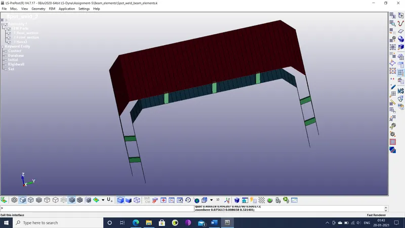
Figure 5: Spot weld solid elements

28. A new solid section is defined for the solid elements generated with element formulation 1 (constant stress solid element).
29. A new node set is created for the solid elements that is then used in a new contact that is created by editing the CONTACT>SPOTWELD keyword.
30. Steps 19-26 are repeated for the second file.

Results: The following observations were made from the animations and plots: -

1. The cross-sectional forces are plotted below.

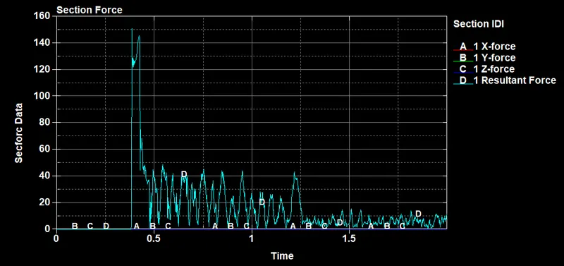
Figure 6: Cross-sectional forces in beam element iteration

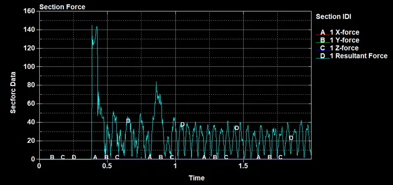
Figure 7: Cross-sectional forces in solid element iterations

It shows that the amplitude of the oscillating forces drop noticeably in the beam element iteration shortly after the beam elements fail. This could be attributed to the relatively higher cross-sectional area of the beam elements compared to that of the solid weld elements, which allows the beam elements to absorb more energy.

2. The axial forces in the weld elements for both iterations are plotted below.

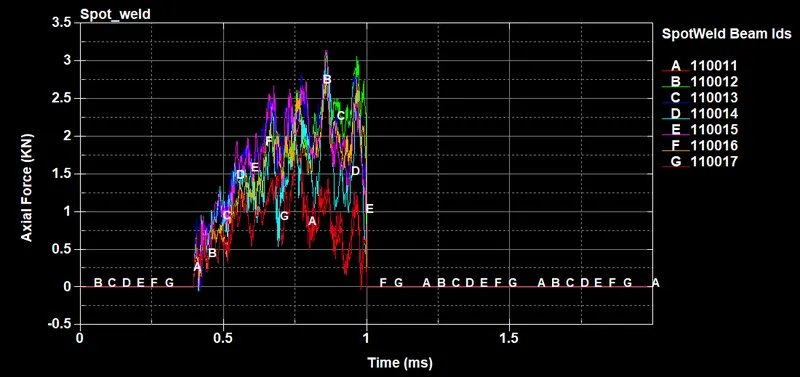
Figure 8: Axial forces in beam elements of welds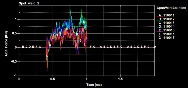

Figure 9: Axial forces in solid elements of welds

Both plots show vibrations in the weld elements that gradually rise and then fall slightly before the welds fail at time t=1ms. This shows the downside of using time as a failure criterion, as one would normally expect such forces to reach a maximum value before failure. In the case of solid weld elements, the overall axial forces are slightly lower and reaches negative values more often.

3. The shear forces in the weld elements for both iterations are illustrated below.

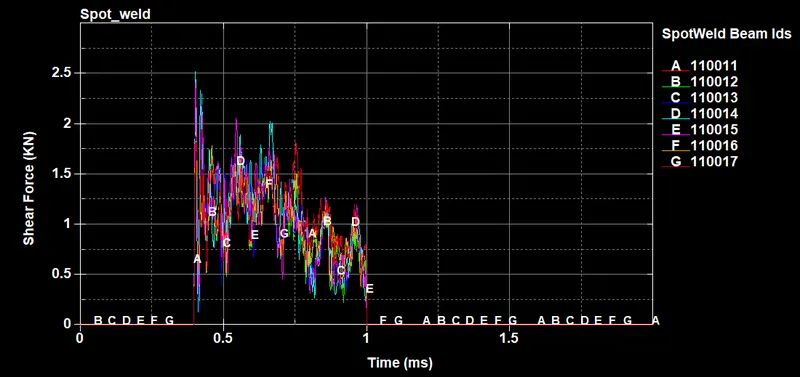
Figure 10: Shear forces in beam elements of welds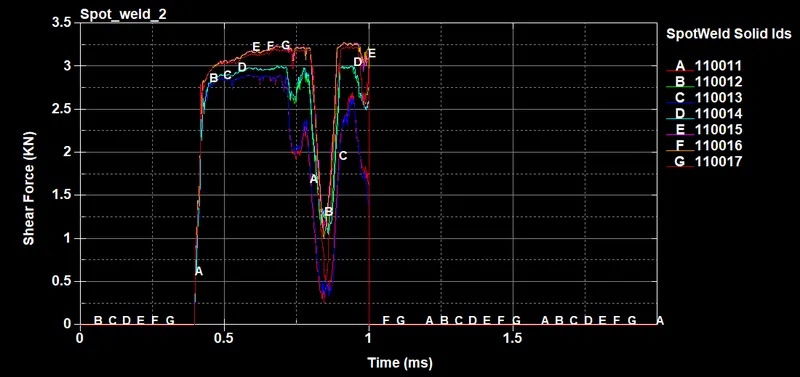

Figure 11: Shear forces in solid elements of welds

They show vastly different behaviors between beam and solid weld elements. In the iteration with solid weld elements, there is a sharp drop in the shear force before failure.

4. The resultant forces on the weld elements are plotted below.

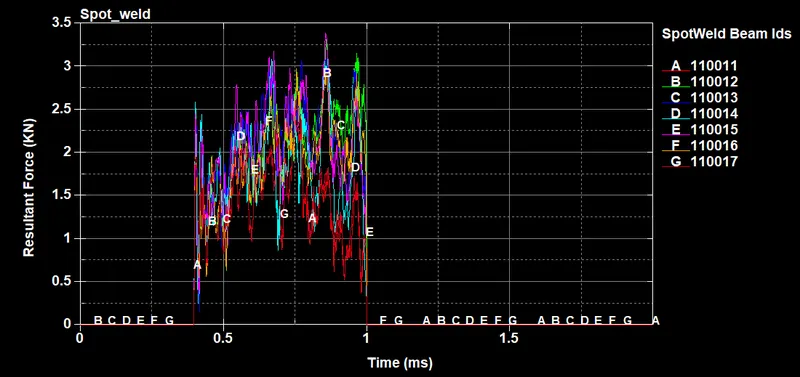
Figure 12: Resultant forces in beam elements of welds

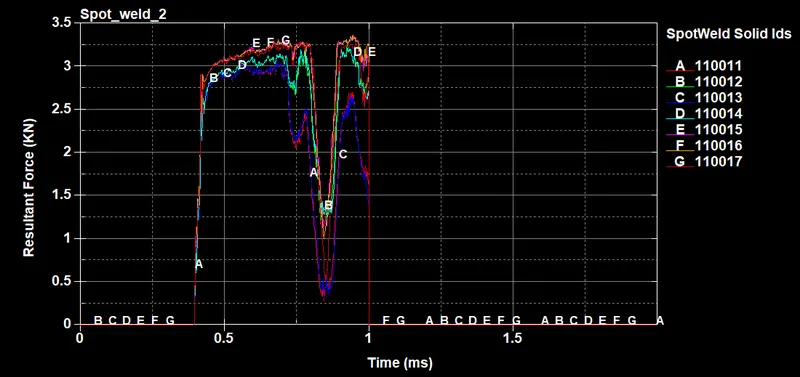
Figure 13: Resultant forces in solid elements of welds

The plots show that axial and shear forces have roughly the same order of magnitude. The solid element force plot shows that the drop in shear force is significant enough to reduce the resultant force.

5. The spotweld length for both iterations are shown below.

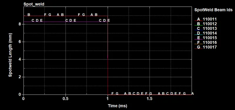
Figure 14: Spotweld length history for beam elements of welds

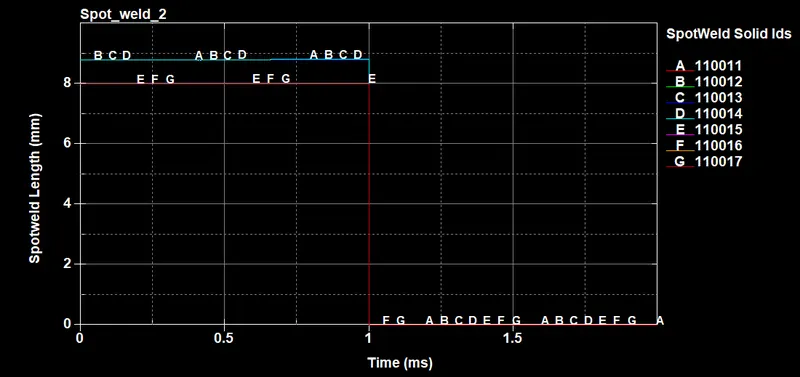
Figure 15: Spotweld length history for solid elements of welds

They show practically no change in weld length, owing to the low forces at the individual welds.

6. The resultant moments for both iterations are plotted below.

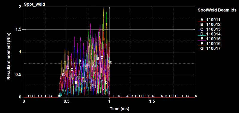
Figure 16: Resultant moment for beam elements of welds

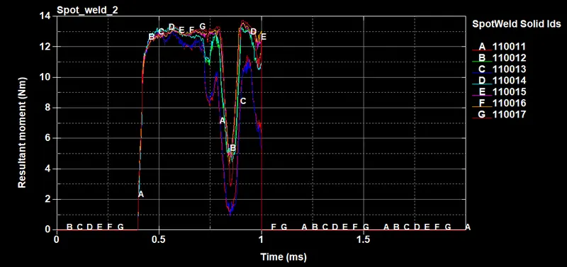
Figure 17: Resultant moment for solid elements of welds

The moment plot for solid weld elements shows the influence of the solid element behavior before failure.

7. The torsion plots for both iterations are shown below.

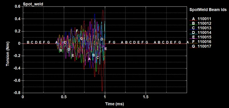
Figure 18: Torsion history for beam elements of welds

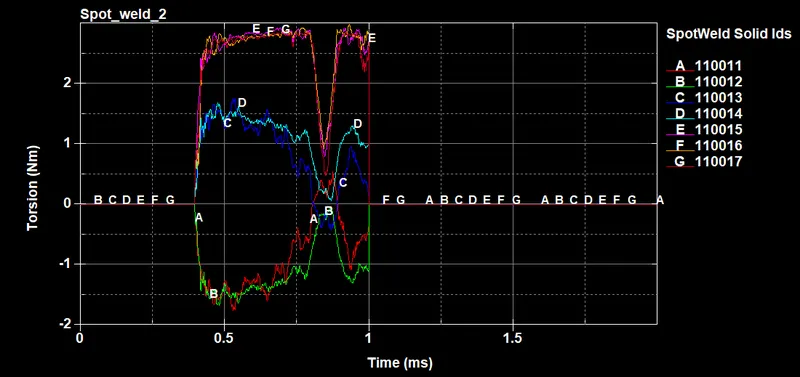
Figure 19: Torsion history for solid elements of welds

It also shows the effect of the solid element behavior before failure. It is more apparent in the solid element plot that torsion is mirrored for welds on opposite sides of the tube.

Conclusion: The given model has been successfully modelled with spot welds and their structural behavior analyzed. A distinct drop in reaction forces and moments were observed in the iteration with solid weld elements, although the reason for this behavior could not be ascertained.