Week 5: Modelling Spotwelds

Aim

To conduct a crash simulation for the given model, two C sections are connected using a series of spot welds, observe and analyze how spot welds and their types can affect the behaviour of the C sections and the impact of their performance.

The specifications and assumptions for the model include the following

• The design features two straightforward rectangular C sections, where a smaller C-section overlaps a larger C-section.
  
  
• C-sections necessitate a series of spot welds for connection. To analyse the outcomes, the spot welds must be executed separately using solid and beam elements.
  
  
• Each spotweld should consist of a single solid element for the solid elements.
  
  
• The same material card, *MAT_SPOTWELD, should be used for beam and solid elements. Steel material data can be applied to the *MAT_SPOTWELD cards, and the failure data should be calibrated based on your results.
  
  
• The C-sections are made of steel, and the simulation will initially use an elastic material model for correctness verification. A nonlinear material card data will be provided later.
  
  
• The model must crash into a rigid wall created using the keyword, 'RIGIDWALL'.
  
  
• The initial velocity of the model is approximately 50 kmph.
  
  
• The unit system used for the simulation is gm-mm-ms.
  
  
• The simulation should satisfy the following condition: An ideal simulation would experience a failure midway through the termination time.
  
  

Output Required

The following deliveries are needed from the simulation:

• Input file (Keyword File).
  
  
• Output files (D3PLOT, GLSTAT, SLEOUT, RCFORC).
  
  
• Final simulation animation.
  
  
• The cross-sectional force, along its length, is generated in the middle of the model.
  
  
• The axial and shear forces between beam and solid elements.
  
  
• The acceleration plot of a node, along its length, is in the middle of the model.
  
  
• The maximum directional stress and strain along the length of a model, such as X-strain and Y-strain.
  
  
• The energy plots comprise Total Energy, Kinetic Energy, Internal Energy, Hourglass Energy, and Sliding Energy.
  
  
• The comparison between the acceleration and stress-strain plots for both cases (spot welds using beam element and solid element).

Procedure

Step 01: Importing And Inspecting The Model

Our goal is to evaluate the impact of spot welds created with beam and solid elements within the simulation. This requires us to replicate the existing model and store it under a different name in a separate location. The procedures remain consistent; the sole distinction lies in the construction of spot welds and their associated processes.

• Model A = Beam element spot welds
  
  
• Model B = Solid element spot welds
  
  

Download the keyword file and save it in a suitable location. Open LS-Prepost and load the keyword file (.K format).

• File >> Open >> LS-DYNA Keyword File >> Select The File >> Open.

Open the keyword manager and understand the model with the assistance of the keyword manager.

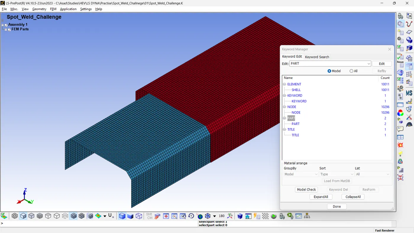
Step 02: Defining Rigid Wall

For the crash simulation, a rigid wall is required where the model will be impacted. The 'create entity' tool can be utilized to define a plane rigid wall. Please note the direction of the head points of the rigid wall. The wall is constructed such that the smaller C section is affected first. This rigid wall is placed with a gap of 10mm to the x-axis with the model.

For the Model A and Model B,

• Model And Part >> Create Entity >> Rigid Wall >> Rigid Wall >> Cre >> Planar >> GeoVector >> 1n+NL (Define vector with 1 node and normal) >> Enable Pick Node and select a node in the edge of the Smaller C Section >> Increase 10 mm to the 'x' value. >> Change the x coordinate of the head point to its negative value. >> Apply >> Done.

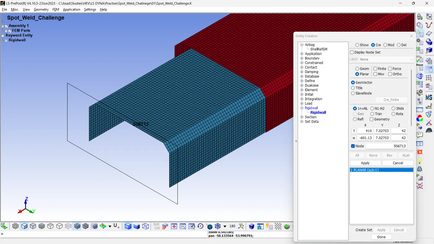
Step 03: Creating Spot Welds Using Beam Elements / Solid Elements

We aim to examine and contrast the effects of spot welds produced using beam and solid elements. This implies that we must create separate beam and solid elements models. A total of seven spot welds have been created between the sections.

For creating the spot welds using the beam elements, For the Model A

• Element and Mesh >> Element Generation >> Beam >> Beam By: Two Node Sets >> Beam >> Pick Node Set 1 and Select The Node From Part 1 >> Pick Node Set 2 and Select The Node From Part 2 >> Create >> Accept >> Done.

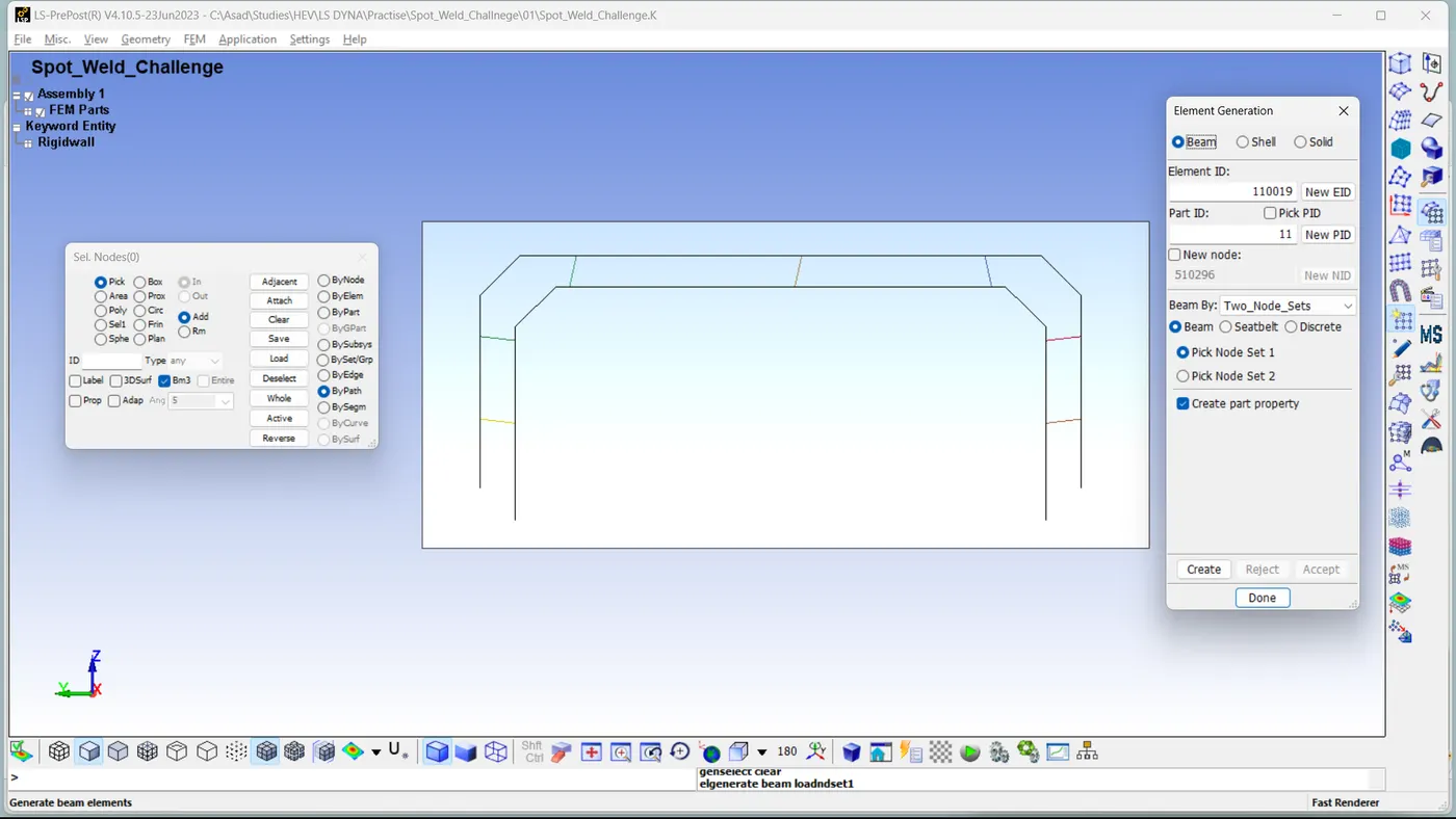
Similarly, using the same nodes, we must create solid elements to replace the beam elements. Save the model with a suitable name. The solid element consists of a single element and it can be created by

For the Model B

• Element Tools >> Element Editing >> Create >> Elem Type: Hexa >> Pick Node 1, Node 2, Node 3 and Node 4 From Bottom Part >> Pick Node 5, Node 6, Node 7 and Node 8 From Top Part >> Accept >> Done

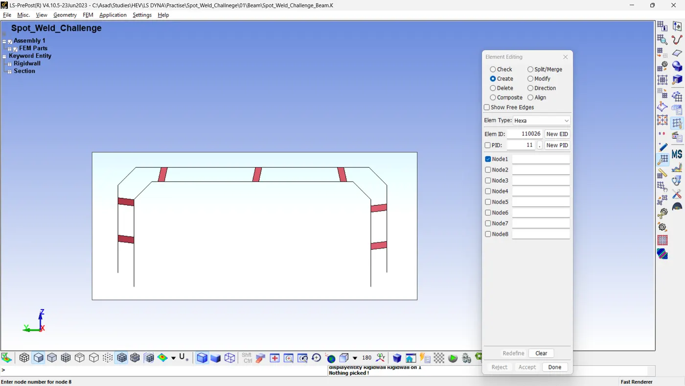
Step 04: Assigning The Initial Velocity

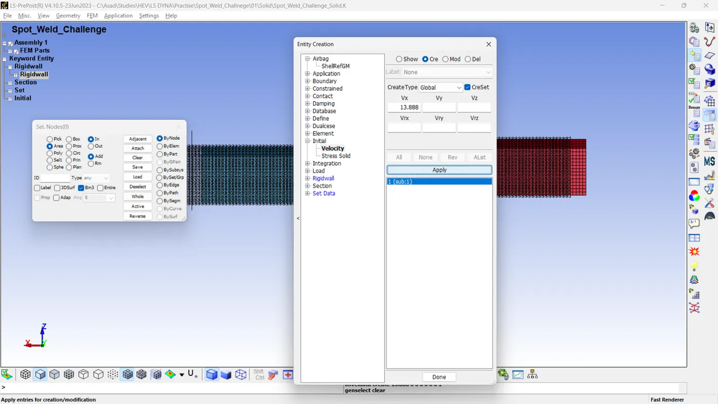
Considering the question, both models have an initial velocity of 50 kmph. If we convert to the 'gm mm ms' unit system the value is 13.888 mm/ms. Therefore, the models are moving at a velocity of 15.333 mm/ms in the direction of the x-axis.

For the Model A and Model B,

• Model And Part >> Create Entity >> Initial >> Velocity >> Cre >> Enable CreSet >> Using Area > Bynode Selection, Select All The Nodes In C Sections >> Vx = 13.888, all other velocity values (Vy, Vz, Vrx, Vry and Vrz) is equal to zero >> Apply >> Done.

Step 05: Defining Materials

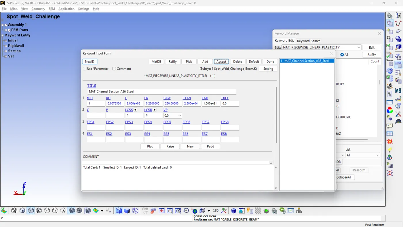
The question indicates that it is constructed from steel. Therefore, a material card with steel properties must be defined. For this purpose, MAT-024 will be utilized. The material properties are based on ASTM A36 Steel.

1. RO= 7.85e-3 gm/mm3
   
   
2. E = 200e3
   
   
3. PR = 0.26
   
   
4. SIGY = 250
   
   
5. ETAN = 25e3

For the models A and B

• Model And Part >> Keyword Manager >> All >> MAT >> 024-Piecewise_Linear_Plasticity >> Give Suitable Title >>Give Appropriate Material Values >> Maintain other values at their default settings >> Accept >> Done.

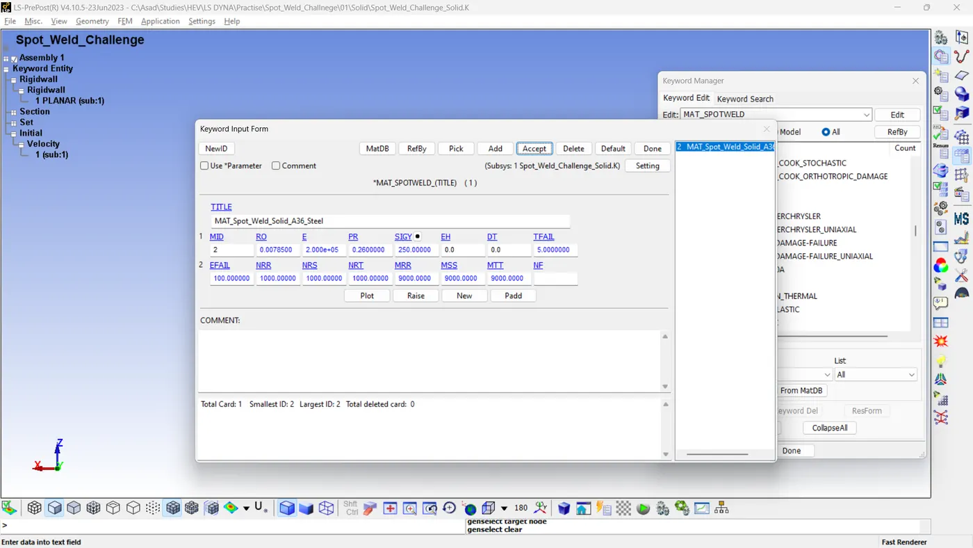
For the spot welds, a MAT-100 card must be added, and the material values should be referenced from A36 steel properties. The Failure Time will be 5 ms and values of moment and forces are given accordingly.

For model A and model B

• Model And Part >> Keyword Manager >> All >> MAT >> 100-Spot_Weld >> Give Suitable Title >>Give Appropriate Material Values >> Maintain other values at their default settings >> Accept >> Done.

Step 06: Defining Sections

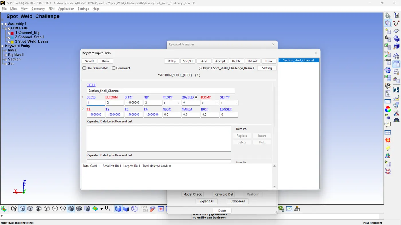
In both models, for the Cs, we need to define a shell section with 1.5 mm thickness and an elform of 2. To create the shell section with default values,

• Model And Part >> Keyword Manager >> All >> Section >> Shell >> Give Suitable Title >> SECID = 1 >> ELFORM = 2 >> T1=1.5 >> Maintain other values at their default settings >> Accept >> Done

For spot welds, we need a beam section for model A and a solid section for model B.

For Model A,

• Model And Part >> Keyword Manager >> All >> Section >> Beam >> Give Suitable Title >> SECID = 2 >> ELFORM = 9 >> CST=1 (For Tubular Section) >> TS1=TS2=1.5 >> TT1=TT2=0 >> Maintain other values at their default settings >> Accept >> Done.

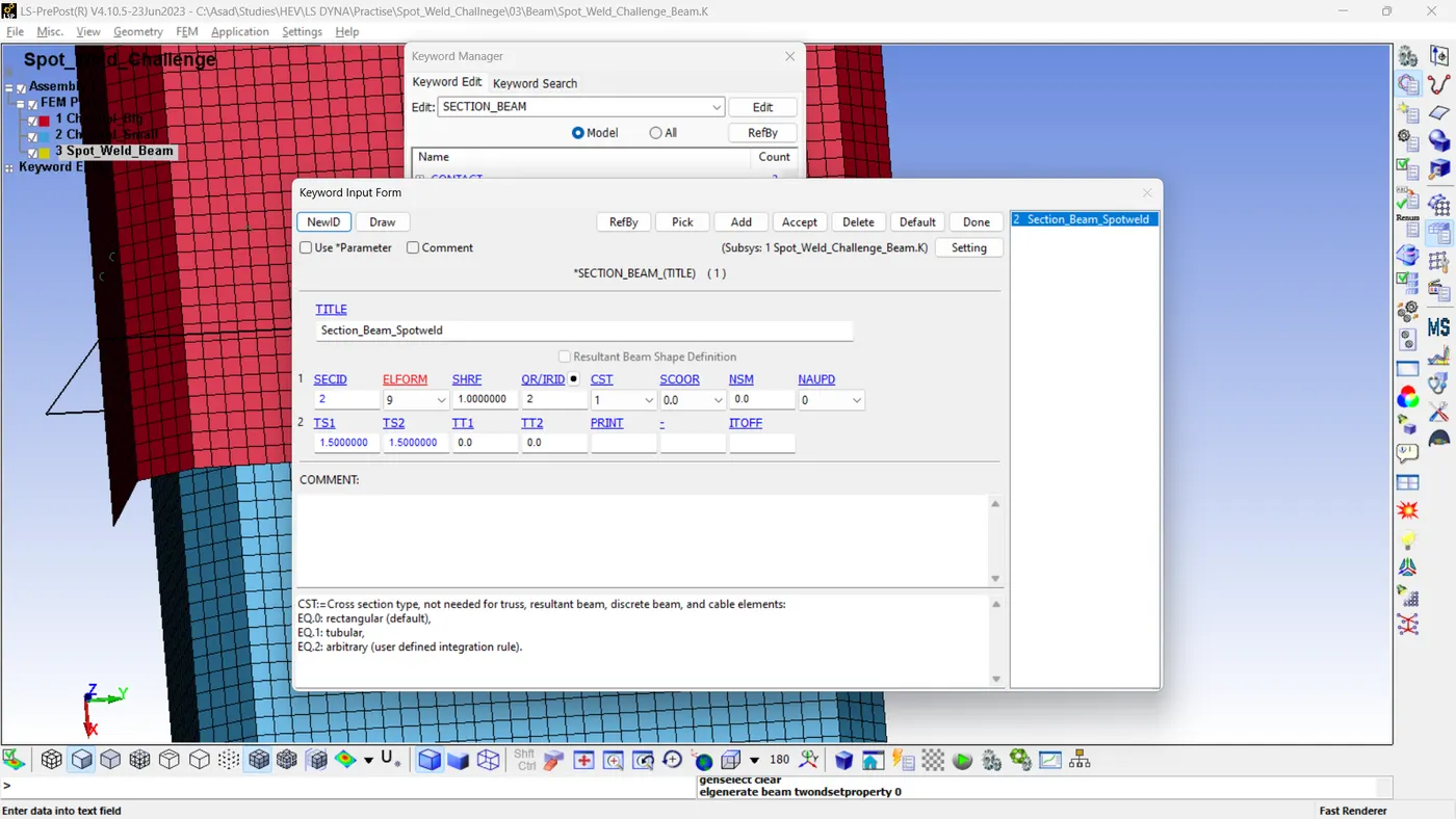
For Model B,

• Model And Part >> Keyword Manager >> All >> Section >> Solid >> Give Suitable Title >> SECID = 2 >> ELFORM = 1 >> Maintain other values at their default settings >> Accept >> Done.

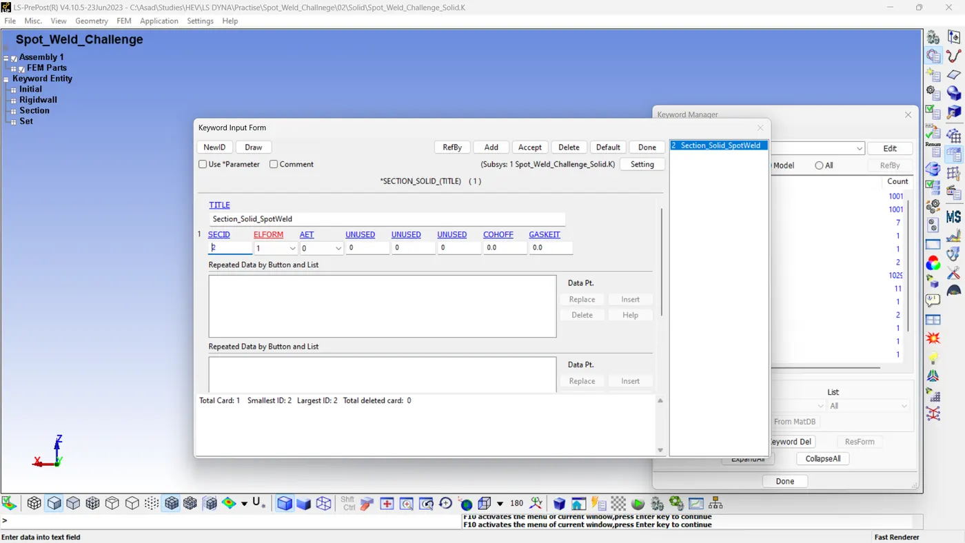
Step 07: Defining Hourglass Card.

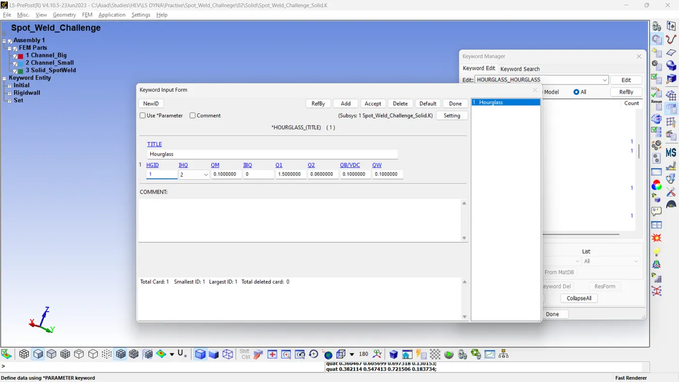
The hourglass card manages the formation of the hourglass energy during the simulation.

For models A and B,

Model And Part >> Keyword Manager >> All >> Hourglass >> Give Suitable Title >> HGID=1 >> IHQ=2 (Flanagan Belytschko Viscous Form) >> Maintain other values at their default settings >> Accept >> Done.

Step 08: Assigning Section, Hourglass And Material To The Parts.

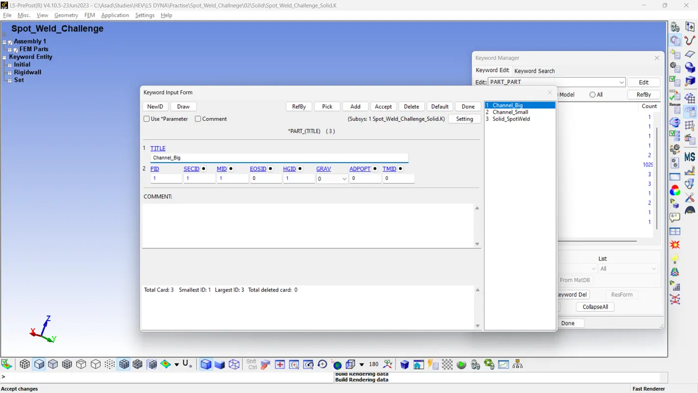
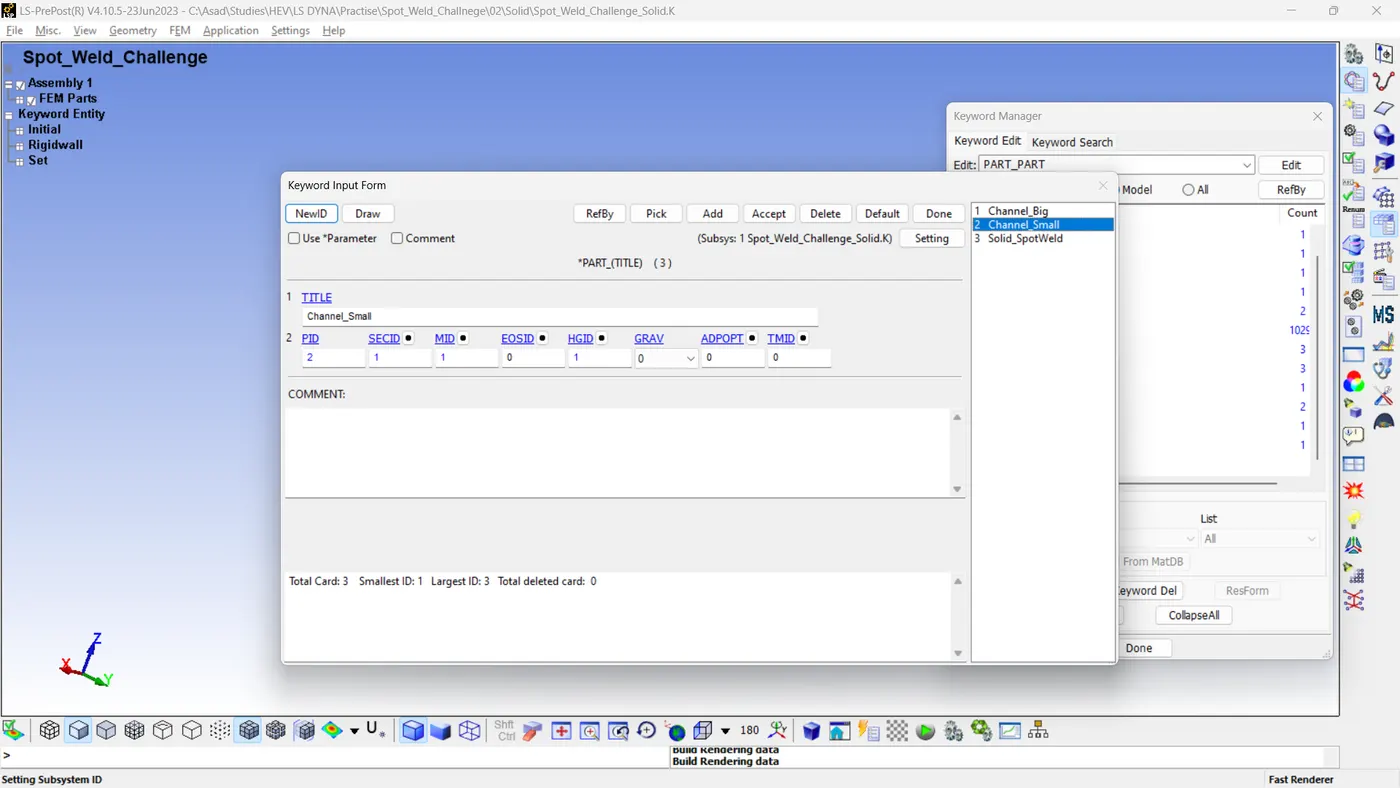
Next, we must allocate specific sections, materials, and hourglasses to each segment of the model.

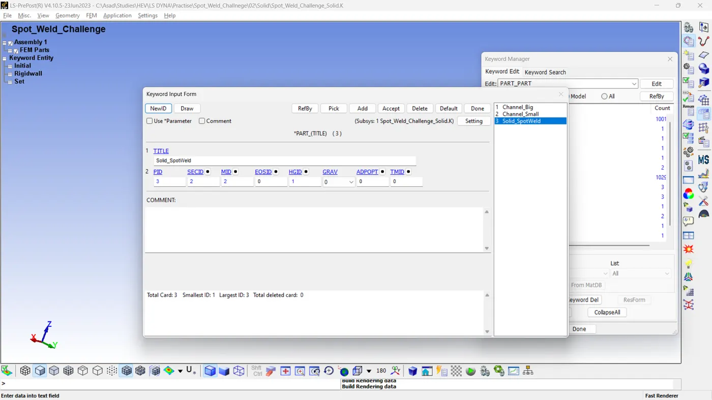
For model A, there are three parts, two shell parts and one beam part. Assign the needed for each part separately.

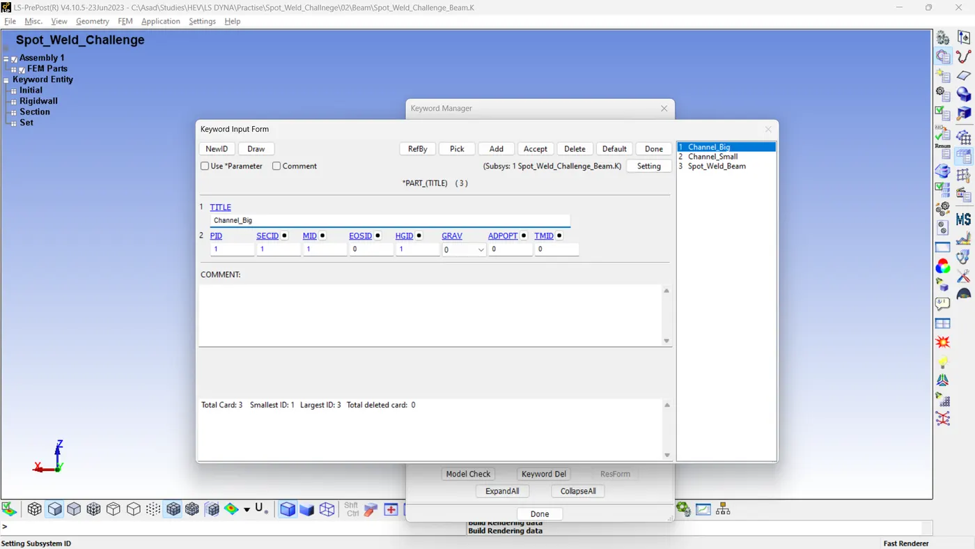
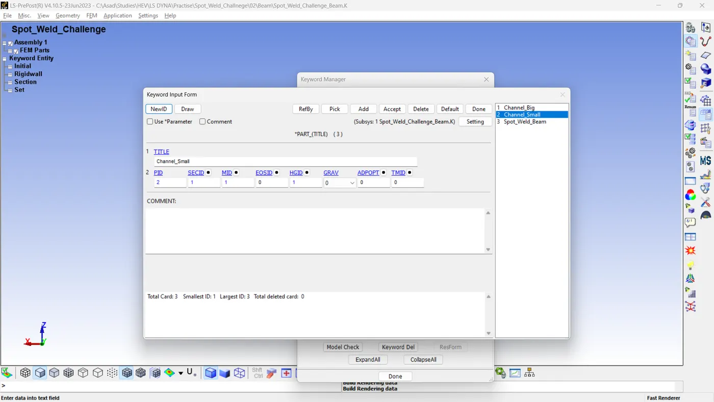
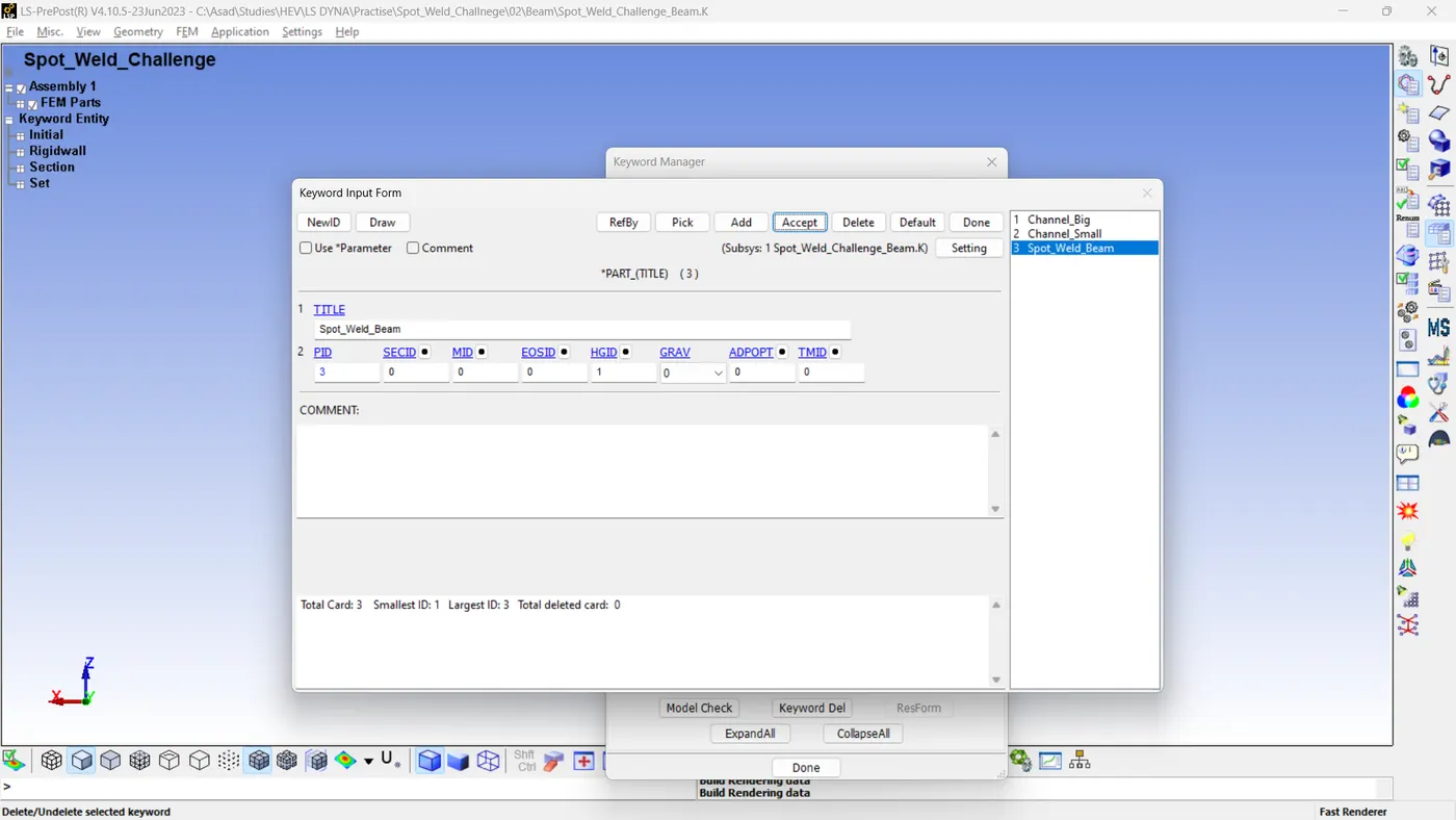
Similarly, for model B, there are two shell parts and one solid spot weld part.

Step 09: Defining Contacts

For the models A and B

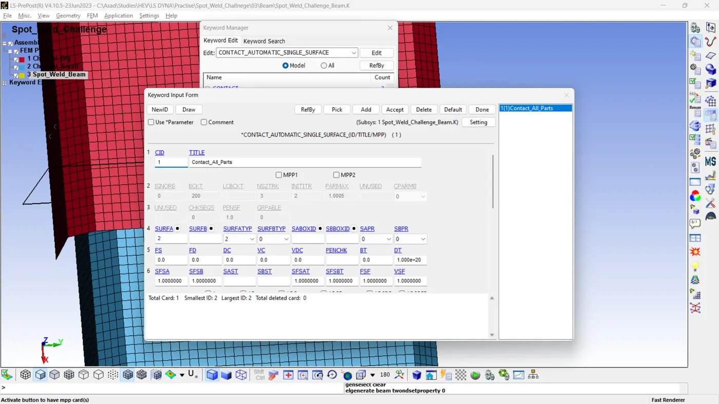
To prevent the penetrations between the parts, we need to define an 'automatic single surface' contact among the elements of the C section. Before proceeding, it is necessary to assemble a part set comprising both C sections and spot welds. Then,

• Model And Part >> Keyword Manager >> All >> Contact >> Automatic_Single_Surface >> Give Suitable Title >> CID =1 >> SURFATYP = 2 (For Selecting Part Set ID as Slave) >> SURFBTYP = 0 (Not Applicable For Self Contact) >> SURFA = 2 (Part Set ID Includes All the Parts) >> SURFB = 0 (Not Applicable For Self Contact) >> Maintain other values at their default settings >> Accept >> Done.

For the models A and B

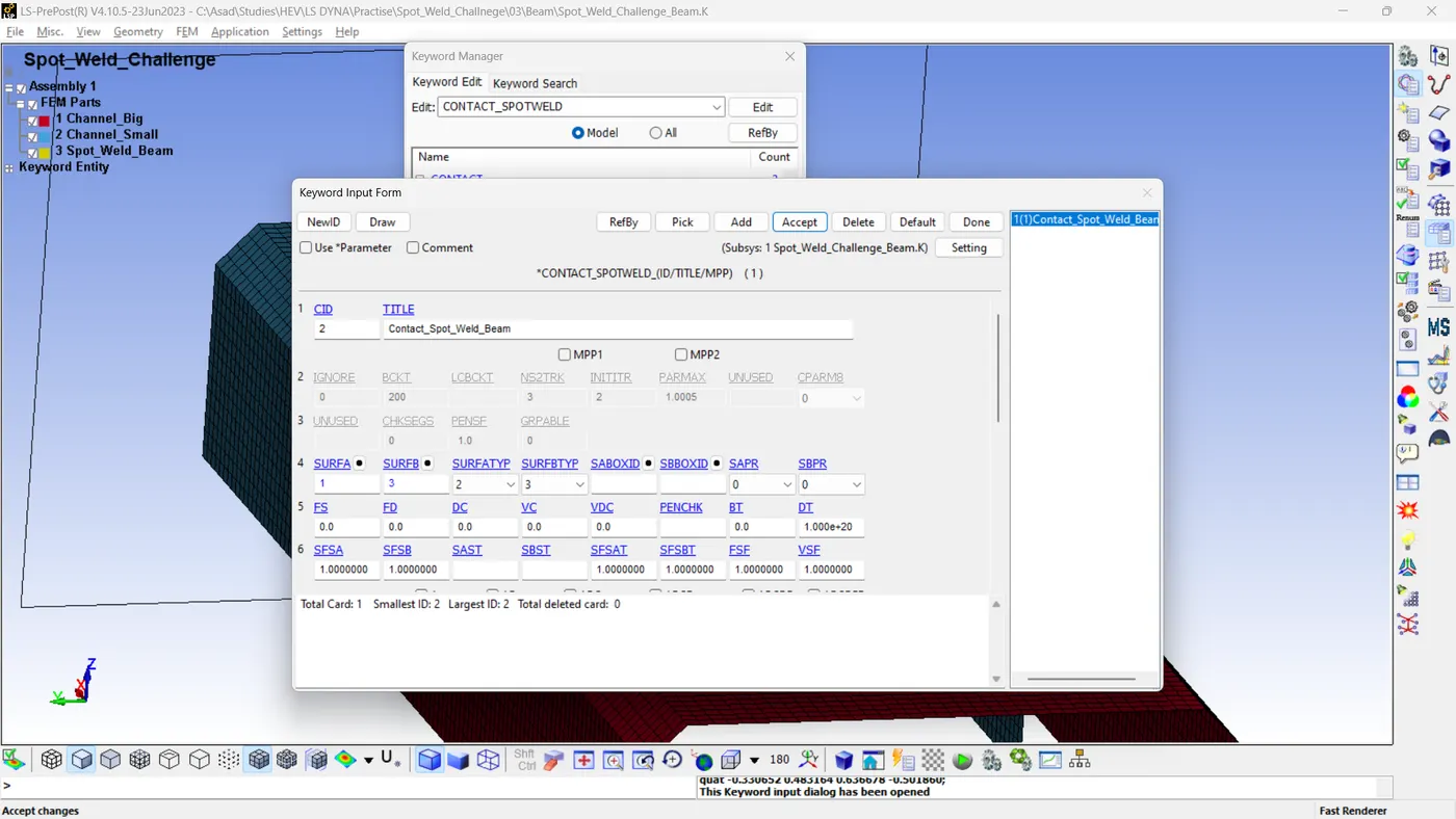
Then, it is necessary to establish contact between the spot weld and C sections. We can use the Contact_Spot_Weld for this purpose. Make a part set that includes both Cs only. Then

• Model And Part >> Keyword Manager >> All >> Contact >> Spot Weld >> Give Suitable Title >> CID =2 >> SURFATYP = 2 (For Selecting C Part Set ID as Slave) >> SURFBTYP = 3 (For Selecting Spot Weld Part ID as Master) >> SURFA = 1 (Part Set ID Includes Cs) >> SURFB = 3 (Part ID of Spot Weld) >> Maintain other values at their default settings >> Accept >> Done.

Step 10: Defining Control Cards

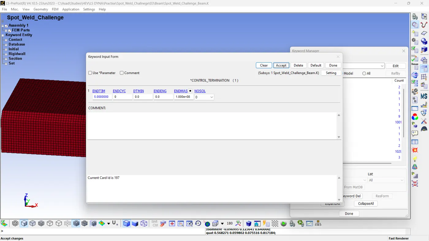
Initially, for both models, it is necessary to define a control card for the termination. The end time will be 5ms

• Model And Part >> Keyword Manager >> All >> Control >> Termination >> ENDTIM =05 >> Maintain other values at their default settings >> Accept >> Done.

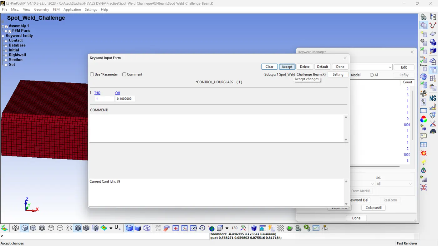
Next, following the same method, we should design a card for the hourglass control.

• Model And Part >> Keyword Manager >> All >> Control >> Hourglass >> IHQ=1 >> Maintain other values at their default settings >> Accept >> Done.

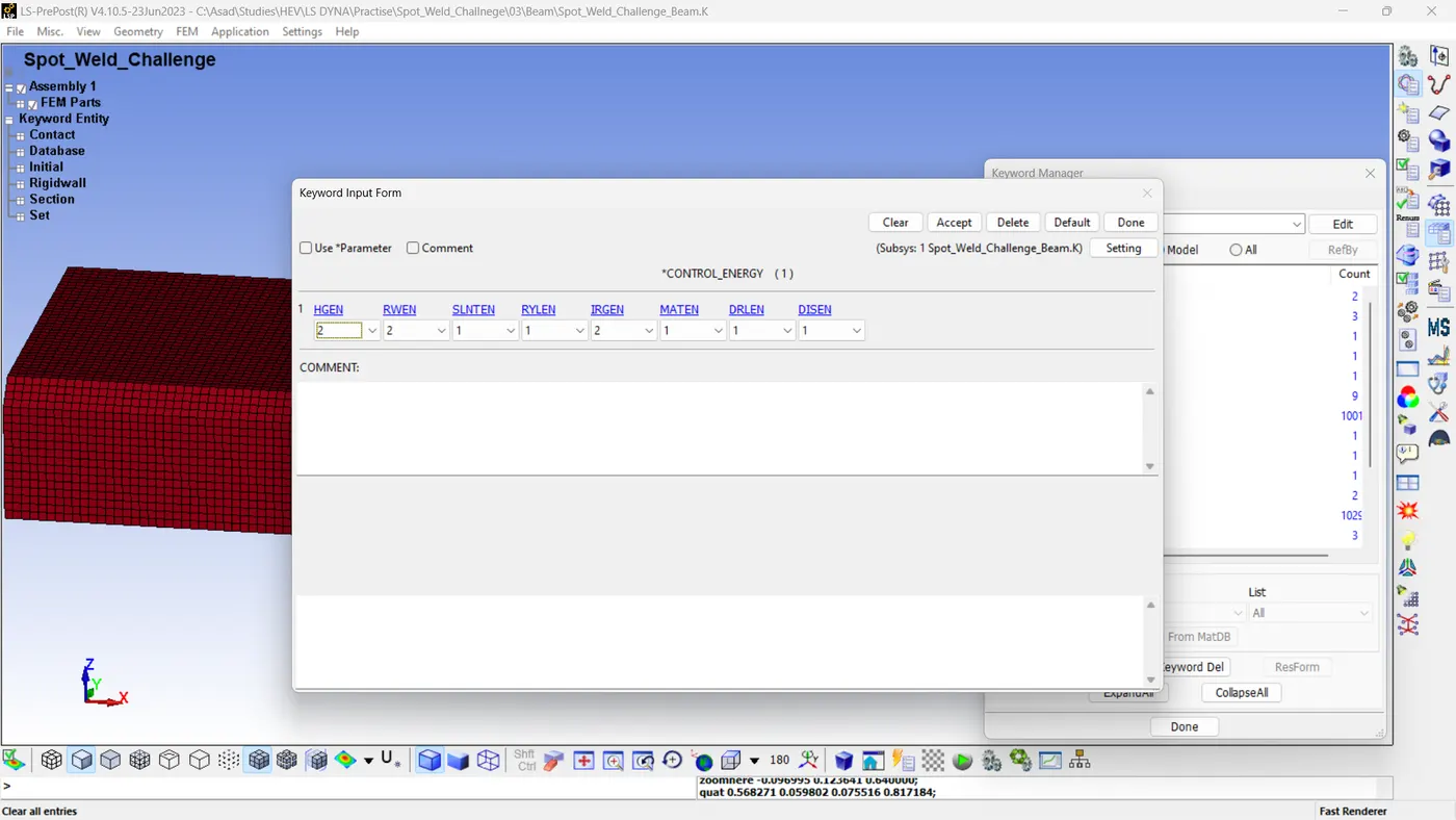
Similarly, we need to assign the control card for energy. For computing the hourglass energy, we need to assign the value HGEN=2

• Model And Part >> Keyword Manager >> All >> Control >> Energy >> HGEN=2 >> Maintain other values at their default settings >> Accept >> Done.

Step 11: Creating Cross Sections

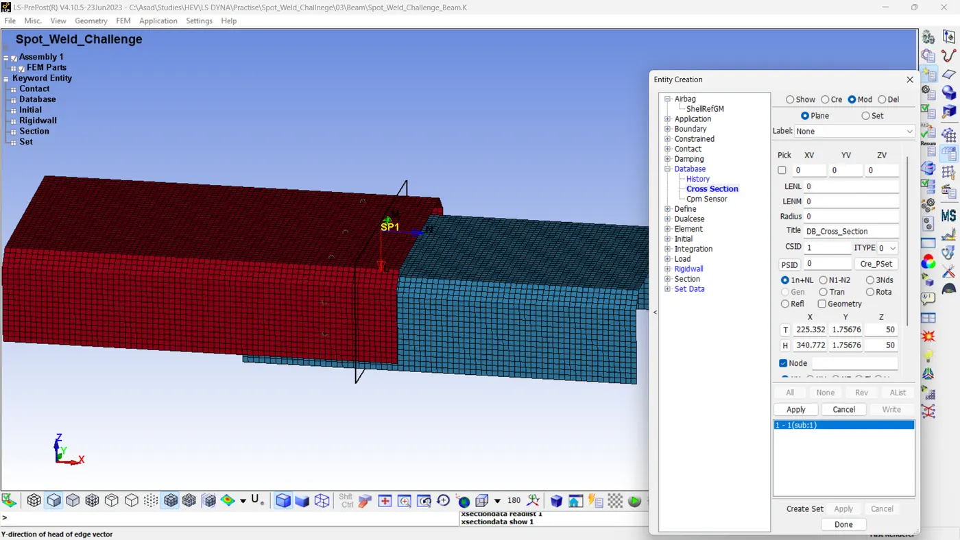
Capturing the cross-sectional force is necessary. To achieve this, a cross-section should be created along the length and situated in the middle region of the model.

• Model And Part >> Create Entity >> Database >> Cross-Section >> Cre >> > Planae >> Give title >> 1n+NL (Define vector with 1 node and normal) >> Pick a node in the mid portion of model >> Apply >> Done.

Step 12: Requesting Outputs

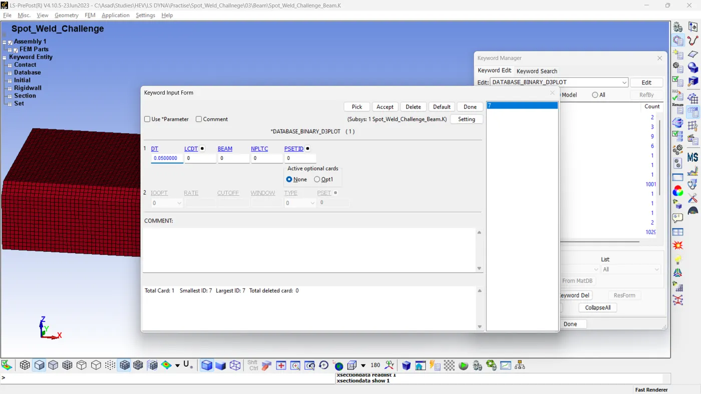
As per the objective, we need D3PLOT as a binary output. To enable that,

• Model And Part >> Keyword Manager >> All >> Database >> Binary_D3PLOT >> DT=0.05 >> Maintain other values at their default settings >> Accept >> Done.

To obtain ASCII outputs, it is necessary to request the outputs for the GLSTAT, MATSUM, SECFORC, SPCFORC, SLEOUT, and RCFORC databases. Also, enable NODOUT output for finding the nodal accelerations.

• Model And Part >> Keyword Manager >> All >> Database >> ASCII_Option >>Select The Database Cards >> DT=0.05 >> Maintain other values at their default settings >> Accept >> Done.

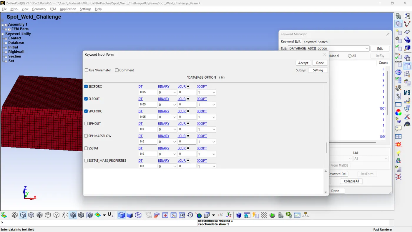
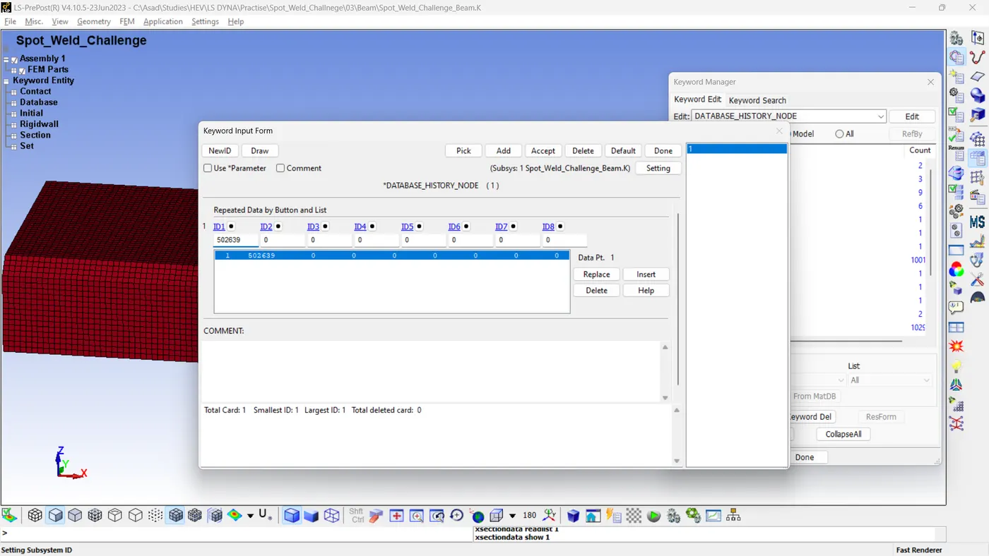
Also, we need to enable the History_Node database to access the nodal properties. Here we take the node ID 502639 for the analysis. For that,

• Model And Part >> Keyword Manager >> All >> Database >> History_Node >> Enter node ID, ID1 =502639 >> Accept >> Done.

Step 13: Model Checking And Simulation For Each Case

Model checking should be finalized, and any errors identified within the model must be resolved. For both models, some warnings can be disregarded, allowing us to continue with the simulation.

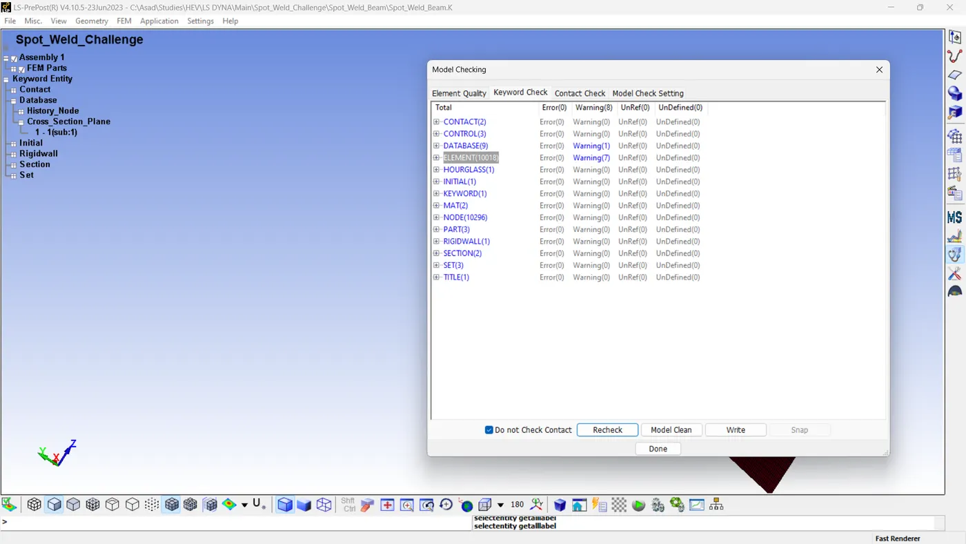
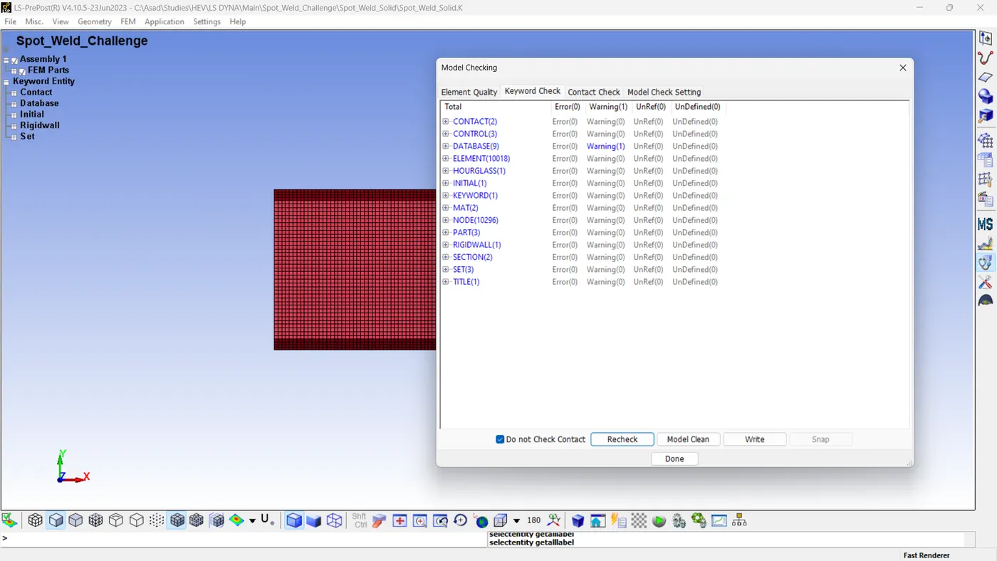
Proceed to save both files using an appropriate name, including the '.K' extension. Then Run the simulation.

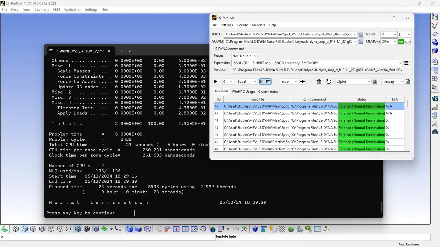
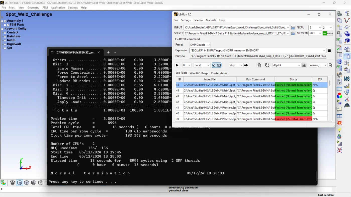
The run time for Model A is 23 seconds and for Model B is 18 seconds.

Results

1) Model A- Spot Weld With Beam Elements

By analysing the simulation animation, Initially, the smaller C section impacted the rigid wall and then bounced back. The larger C-section is joined to the smaller C-section using seven beam spot welds. Both sections share the same initial velocity and direction. When the smaller section rebounds, it tugs on the larger section via the spot welds, resulting in deflections in both components and causing them to fold against each other. After the smaller C section rebounds, the beams will initially pull on the larger C section, causing both to deflect and altering the trajectory of each part. Additionally, the smaller C-section collided with the rigid wall once more as an effect of the beam and bigger C-section. The spot welds also cause a decrease in their velocities. It didn't stop the parts and the beam elements failed and broke resulting in more deflection. At the end, the tip of the larger section opens outward, while the smaller section closes inward.

1. Directional Stresses Along X Axes, Y Axes And Von-Mises Stress

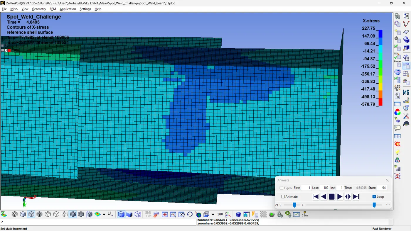
The stress acting on the x-axis is depicted in the images below.

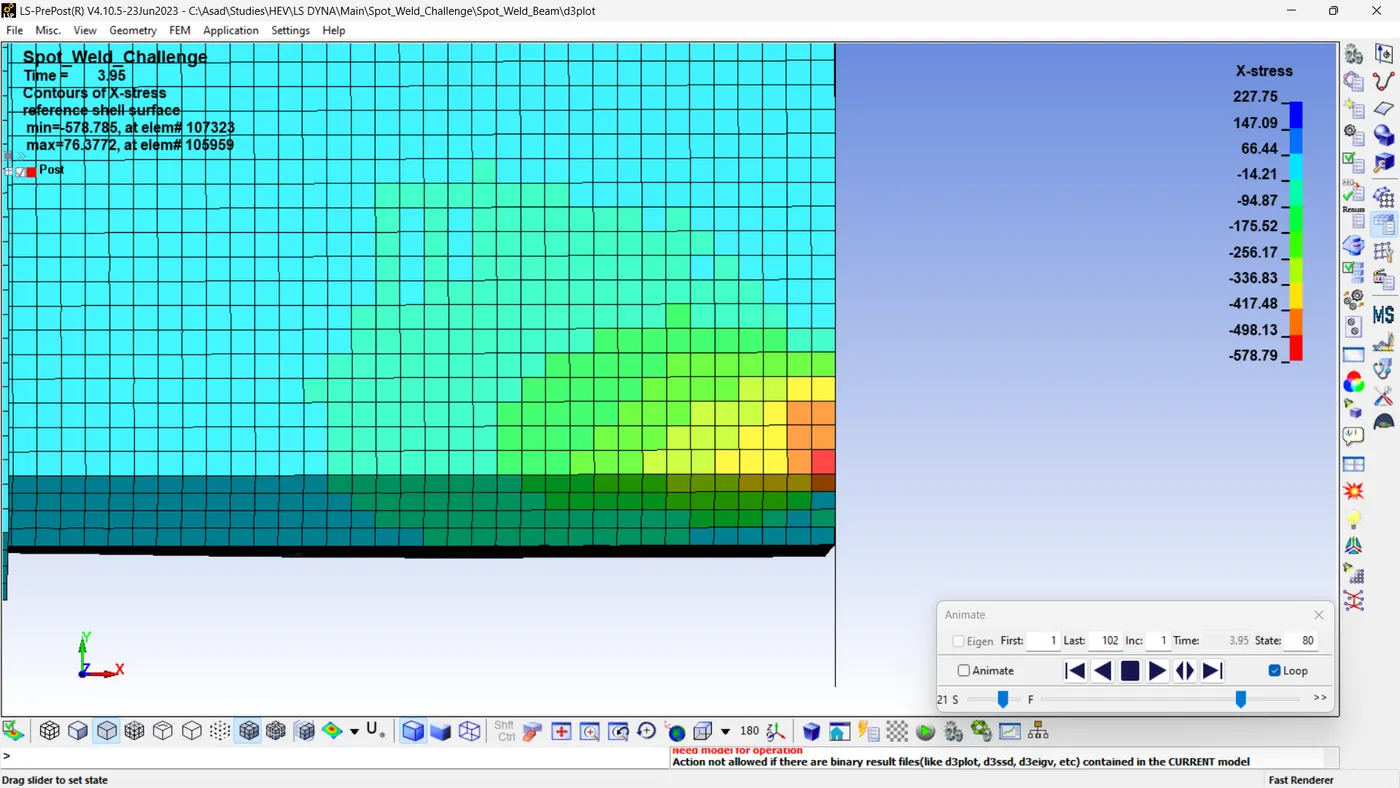
• When the smaller section rebounds against the rigid wall for the second time, the combined mass and velocity of the larger C section result in a maximum compressive stress of 578.79 MPa at 3.95 ms. The affected elements are located along the edge of the smaller C-section where it contacts the rigid wall.
• Subsequently, as a result of spot welds, the region in the middle part of the smaller section experiences a peak tensile stress of 227.75 MPa at 4.6495 milliseconds.

The stress acting on the y-axis is illustrated in the images below.

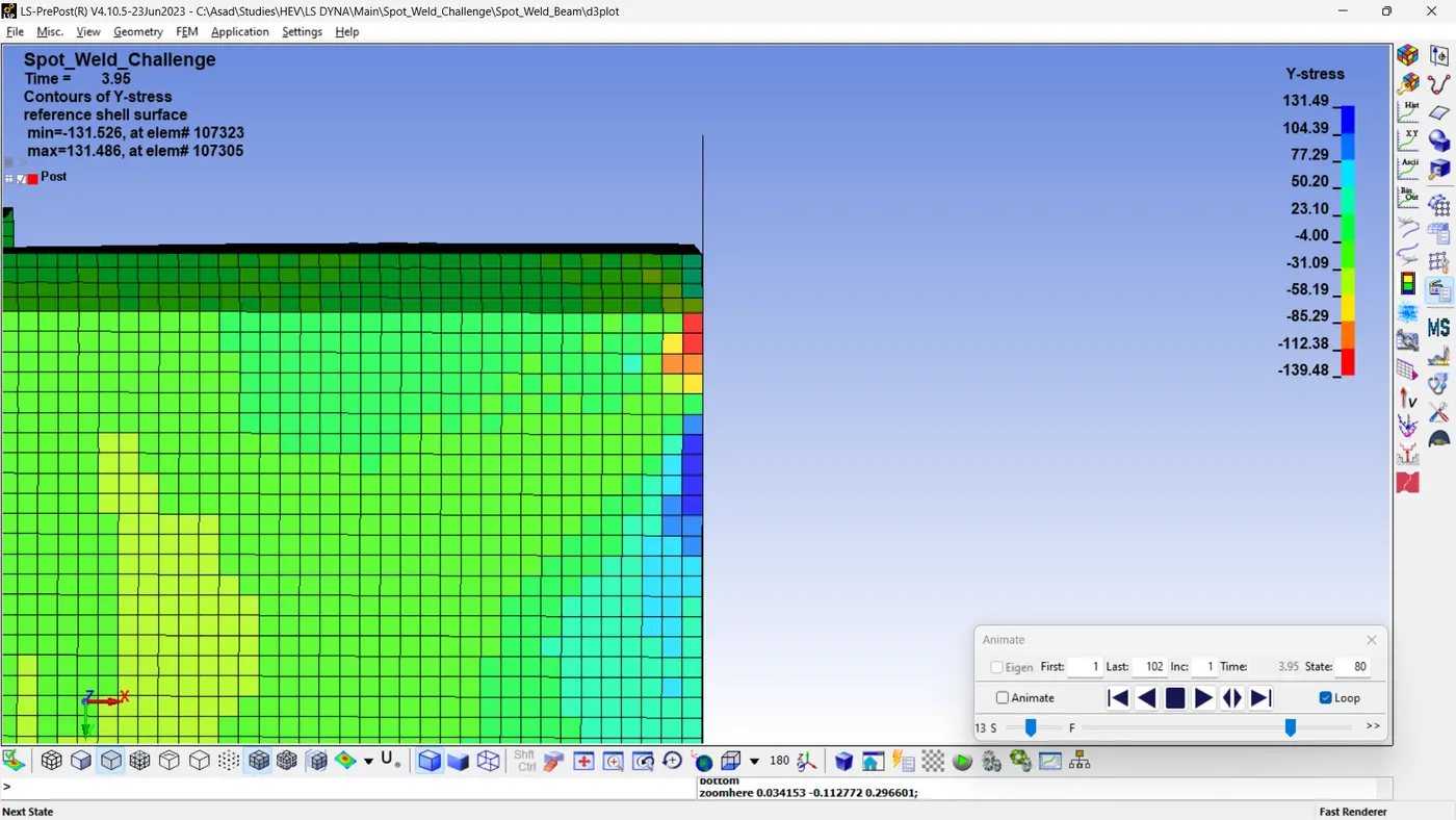
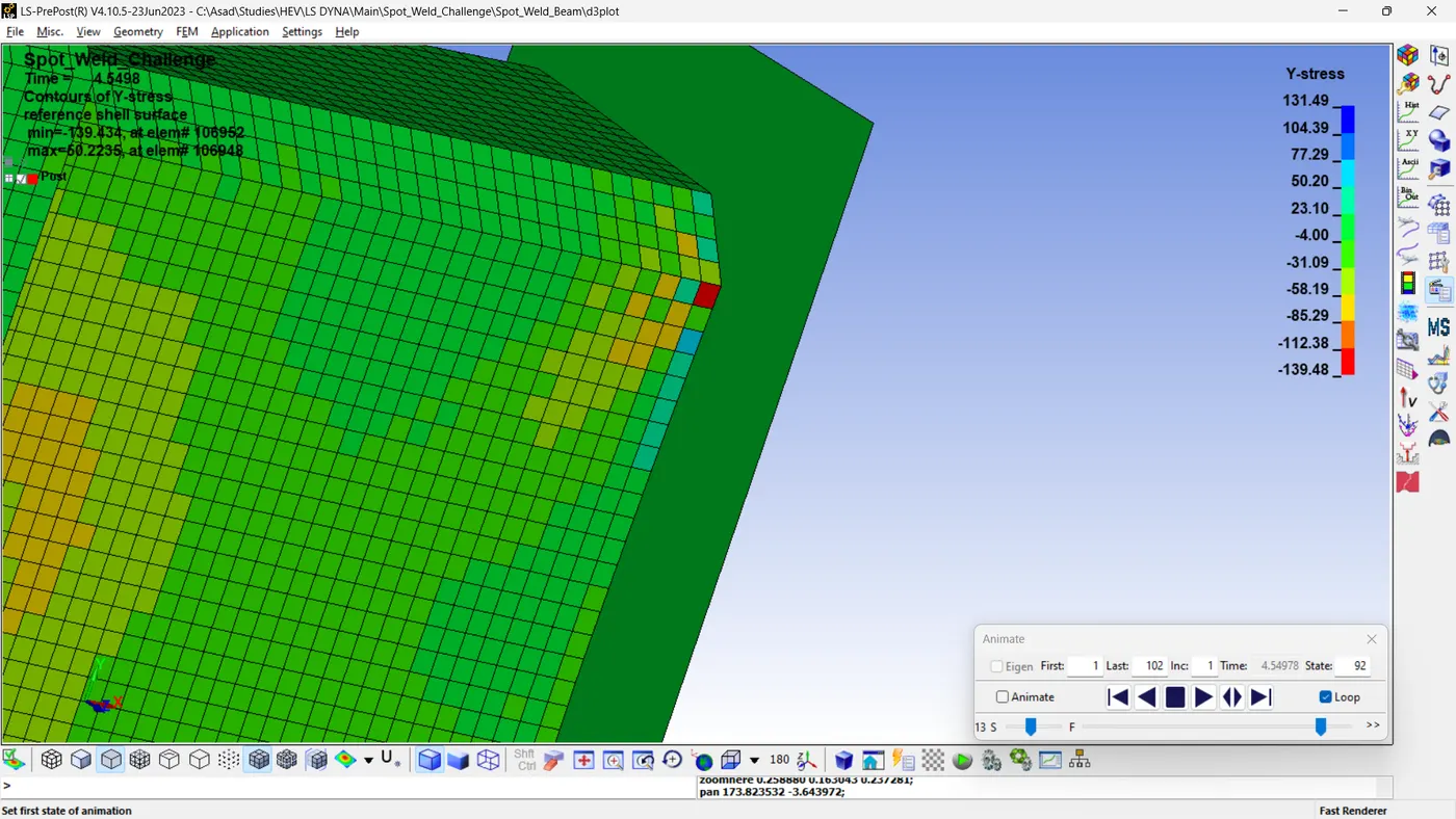
• The maximum compressive stress value occurs on the y-axis at 139.48 MPa at 4.5498 ms, and the tensile stress reaches 131.48 MPa at 3.95 ms. The impacted elements are situated at the periphery of the smaller 'C' section, where contact is made upon the occurrence of the second impact.

The effective stress can be represented using the Von Mises stress.

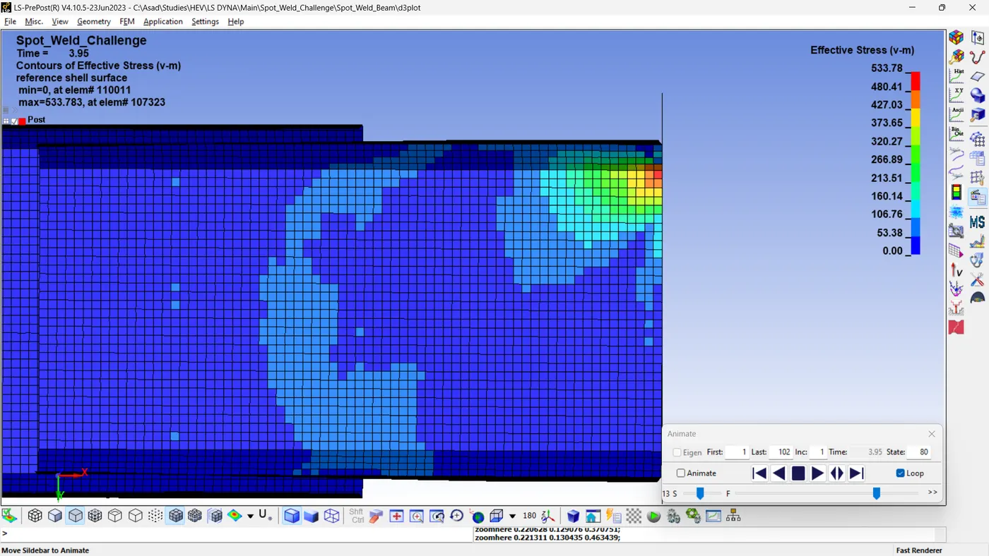
• The value of maximum Von Mises stress is equal to 533.78 MPa. The animations reveal that the elements surrounding the spot weld are also impacted during the simulations. Nearly all the stress distributions are focused on the smaller section, with the maximum stress occurring after the second impact, located close to the point of contact.

2. Strain Along X Axes, Y Axes And Von Mises Strain.

The strain along the X and Y axes, as well as the effective strain (Von Mises), are depicted below.

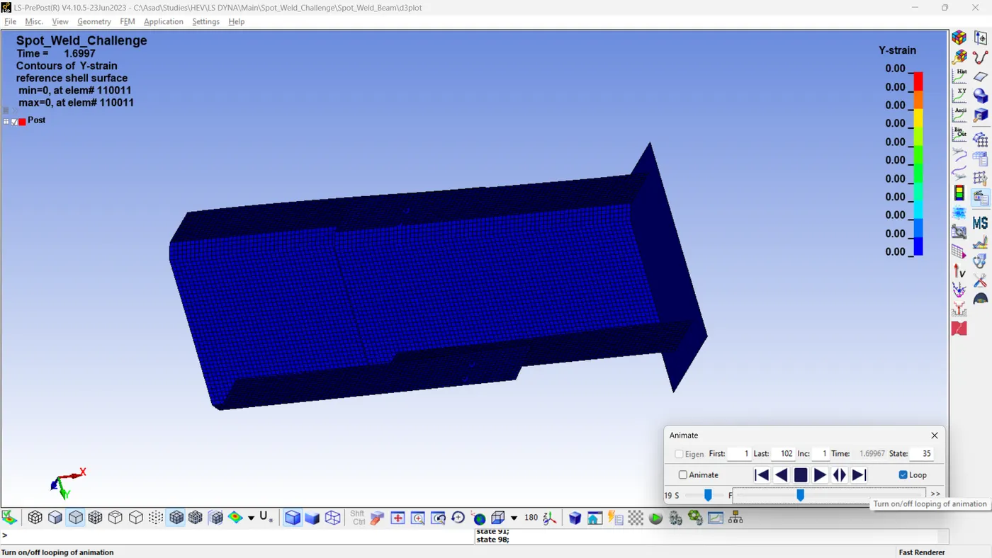
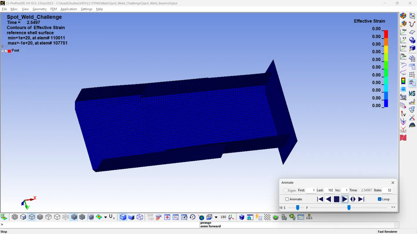
The simulation indicates that the X, Y and Von Mises strain values remain at zero.

3. Global Energies

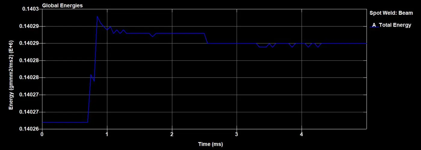
The various energy plots and their observations are mentioned below.

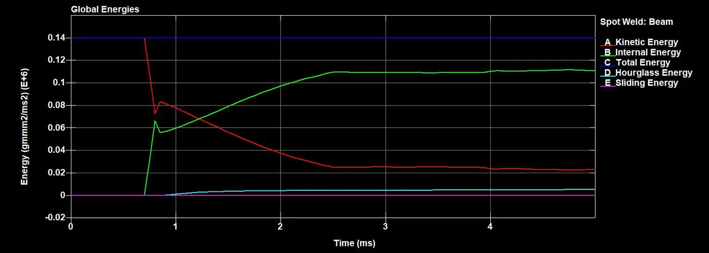
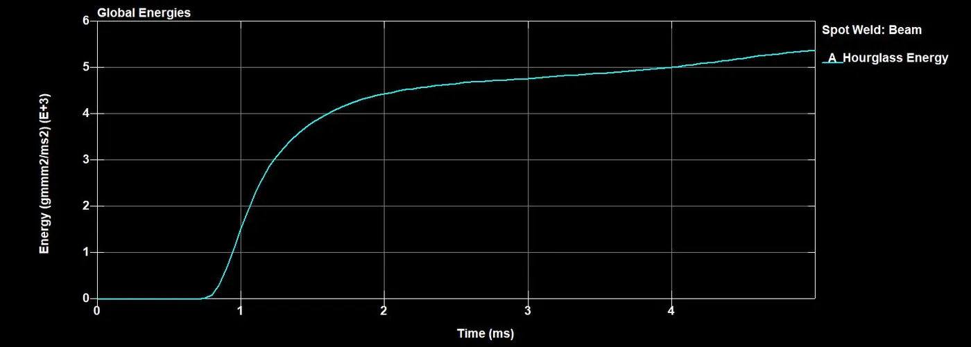
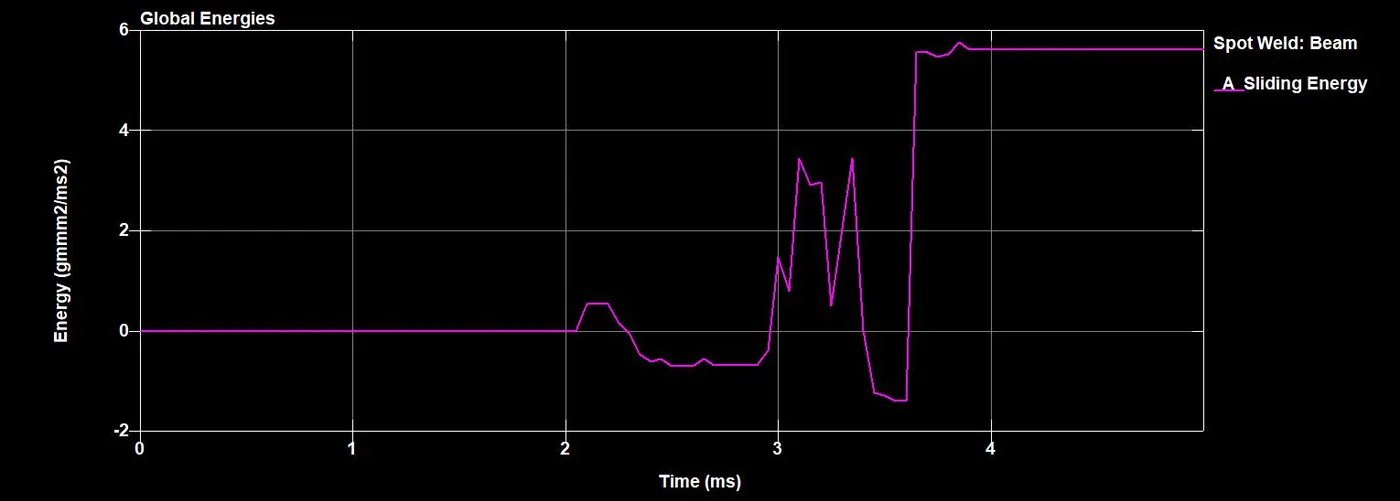
• The KE reaches a maximum value of 1.40e5 within the first 0.699 seconds, which is attributable to the initial velocity of the model. When the contact occurs, KE is converted to PE, so there is a rapid decrease in KE down to (7.29e4) due to this impact. Then it rebounds, and that velocity results in a slight increase in KE (8.36e4) After the model begins moving toward the wall and impacts it, there is a nearly uniform decrease in kinetic energy to 2.53e4 within 2.5ms. Then, the subsequent rebound results in a slight decrease until the end of the simulation.
  
  
• In the IE, the opposite of what occurs above takes place. The IE remains zero until the impact begins. At the time of the collision, the IE instantly increased its value to the maximum value (6.69e4) and The value then rapidly decreased to 5.59e4, The subsequent rebound motions resulted in a uniform increase in potential energy (PE), followed by a slight increase in PE due to the second rebound.
• The intersection of these plots suggests that deformation is taking place.
• The entire crash's Total Energy (TE) initiates at 1.40e5. As the crash commences, there is a slight increase in energy, followed by a gradual decline.
  
  
• Hourglass energy (HE) is not produced until the onset of the crash. The impact initiates the HE and gradually increases the value (more of a parabolic increase) (5.83e3) until the end of the simulation.
  
  
• The sliding energy is zero up to 2.05ms. Then, when both C sections begin to contact each other, sliding energy is produced. Following multiple variations, the sliding energy peaks at a value of 5.78. This stays consistent for the duration of the simulation.

4. Cross-Sectional Force

The sectional force for the mid-section of the crash box is illustrated below.

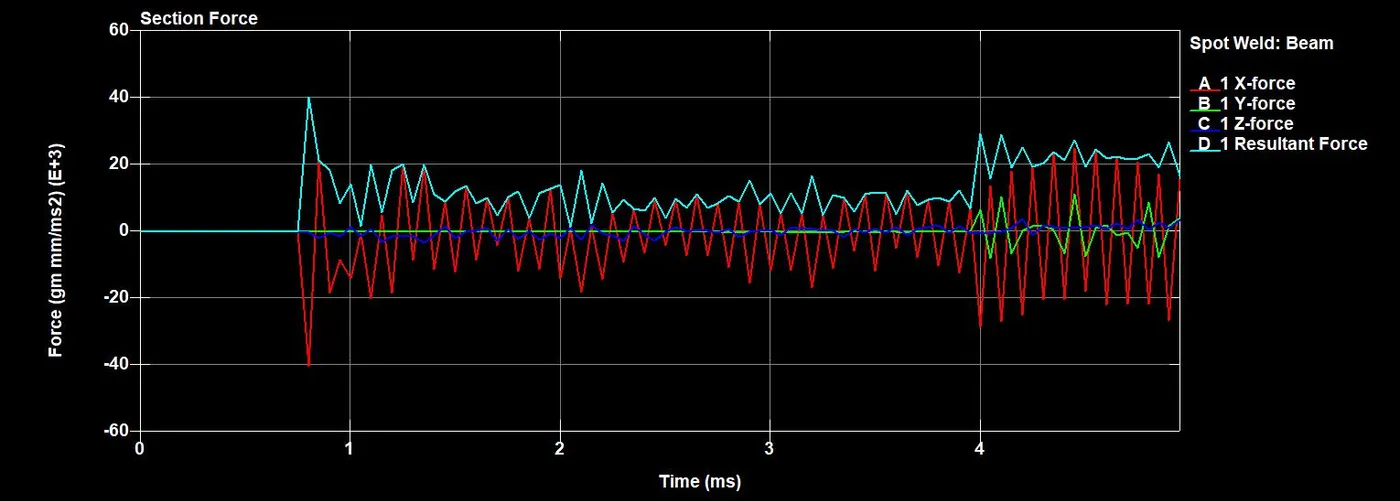
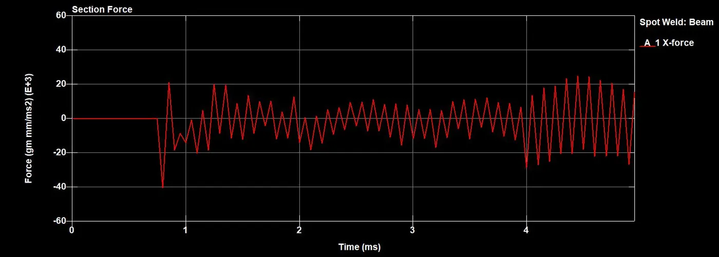
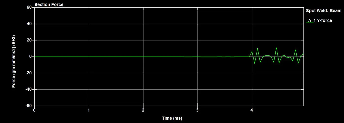
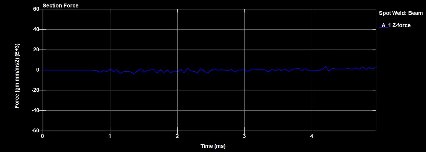
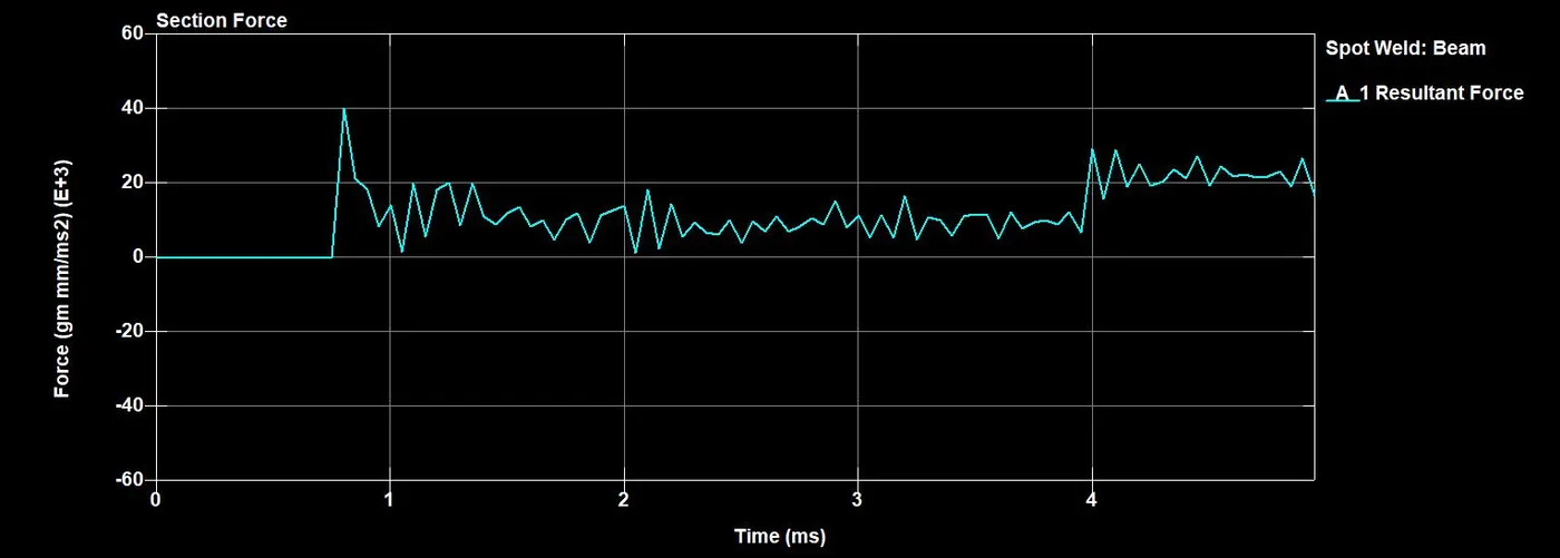
• The cross-sectional force in the x-direction is significantly higher than the forces on the y and z axes. The resultant forces remain at zero until the impact occurs. At the moment of impact, they spike sharply before declining abruptly and fluctuating continuously. Ultimately, we can observe the consequences of the second impact and its subsequent rebound.

5. Nodal Accelerations

The nodal accelerations for the mid-section of node ID 502639 in the crash box are illustrated below.

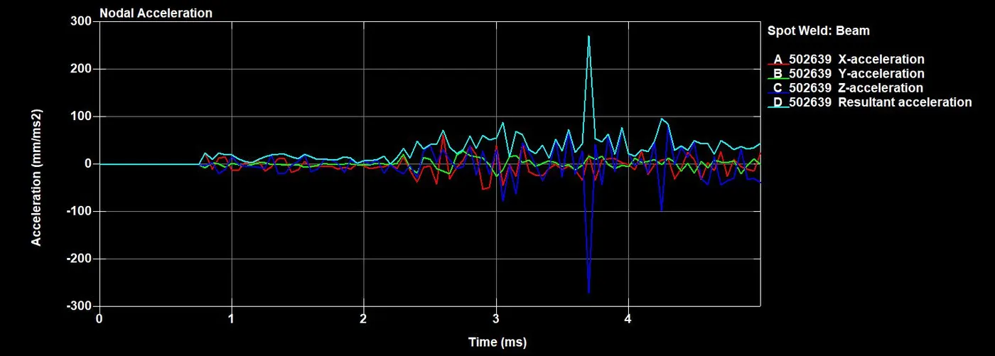
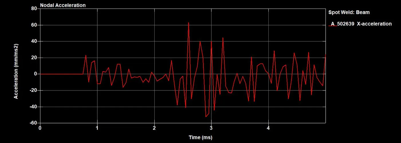
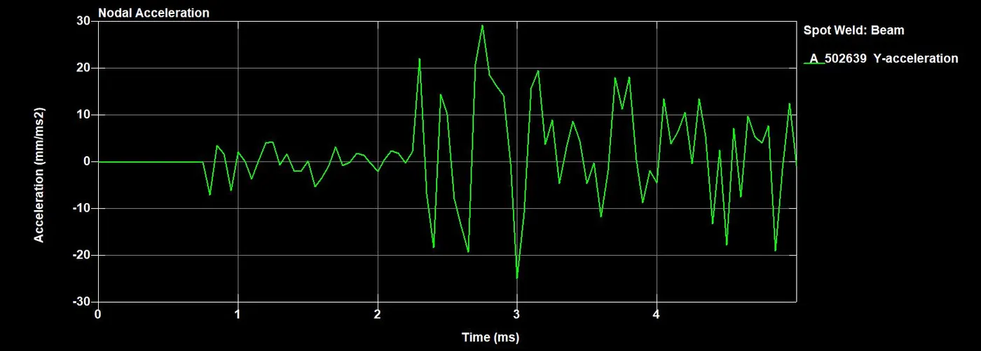
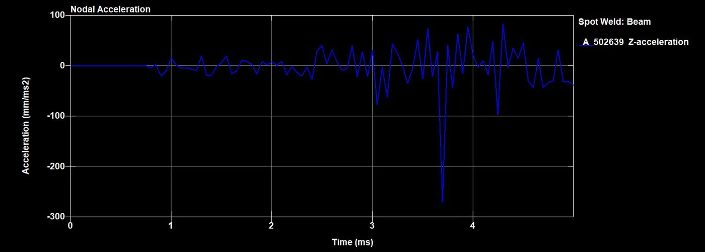
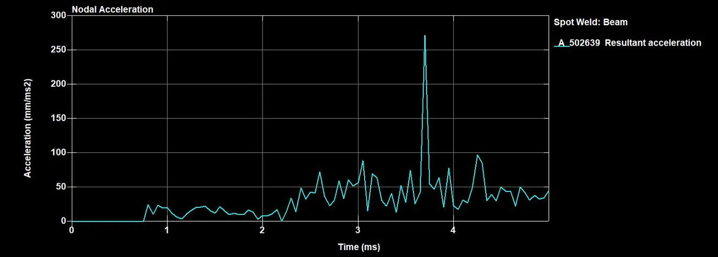
• The nodal accelerations in the x-direction are significantly higher than on the y and z axes. The resultant accelerations stay at zero until the impact takes place. The resultant accelerations stay at zero until the impact takes place. There is a sharp spike to approximately 24.5mm/ms2 at the instant of impact, followed by a sudden decline and continuous fluctuations. The peak acceleration happens almost instantly at about 3.70 ms, reaching up to 272 mm/ms².

2) Model B- Spot Weld With Solid Elements

Similar to model A, in the second scenario, the smaller C section makes contact with the rigid wall and then rebounds. Here the spot welds are constructed using solid elements. When the smaller C-section made contact with the rigid wall, all the spot welds failed, causing both sections to separate from each other. The rebound of the smaller C section does not influence the movement of the larger C section, allowing it to move independently toward the rigid wall.

1. Directional Stresses Along X Axes, Y Axes And Von-Mises Stress

The stress acting on the x-axis is depicted in the images below.

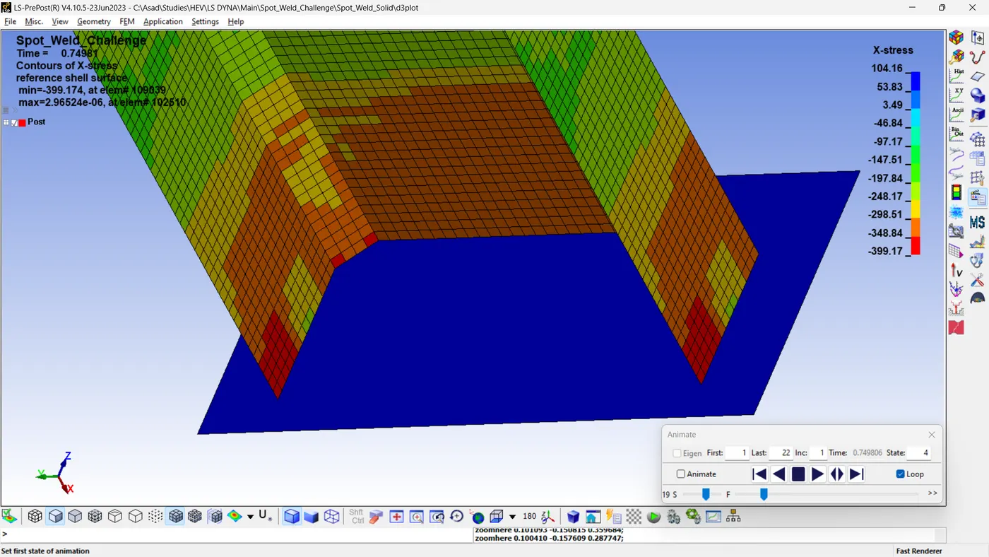
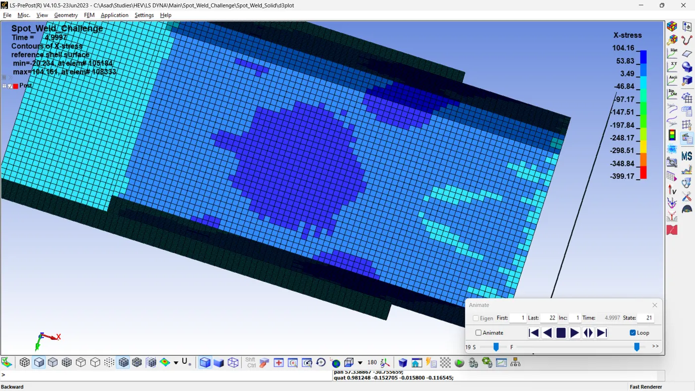
• During impact, the elements making contact with a rigid wall undergo compression. It is observed that the edges of the smaller section (both ends and at the fillet) experience a maximum compressive stress of 399.714 MPa at 0.74981 ms. The stress distribution extends towards the end of the section.
  
  
• The maximum tensile stress is experienced at the mid-portion of the smaller C-section, reaching a peak value of 104.16 MPa at 4.9997 milliseconds.

The stress acting on the y-axis is illustrated in the images below.

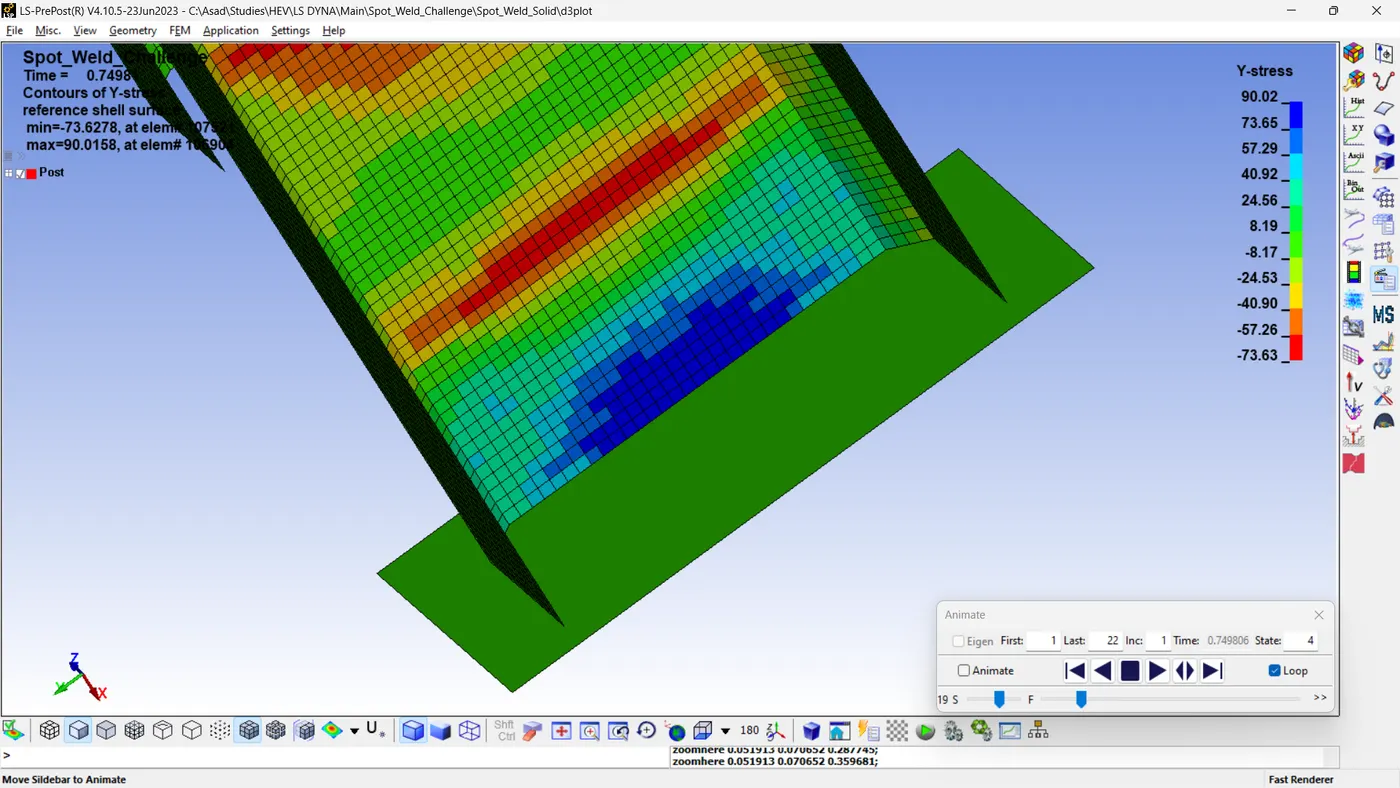
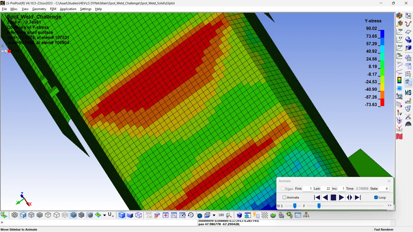
• On the Y-axis, the maximum compressive stress is 90.02 MPa and the maximum tensile stress is 73.63 MPa, both occurring simultaneously. The element undergoing maximum compressive stress is located at the mid-portion of the edge where it contacts the rigid wall. The maximum tensile stress occurred at the midpoint of the smaller C-section.
  
  

The effective stress can be represented using the Von Mises stress.

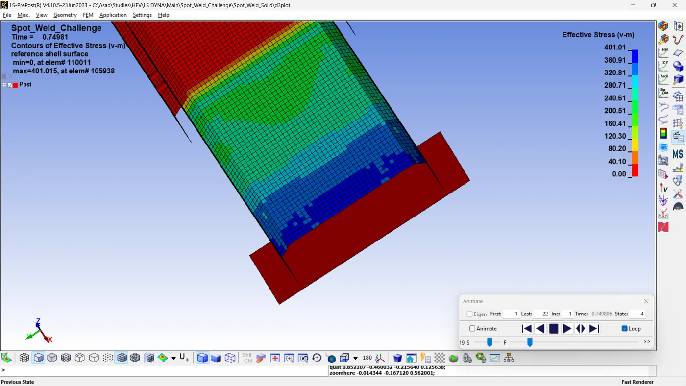
• The maximum Von Mises stress value is 401.01 MPa, occurring at the contact point and then distributing along the length of the smaller C-section. The larger C-section remained unaffected throughout the simulation.

2. Strain Along X Axes, Y Axes And Von Mises Strain.

The strain along the X and Y axes, as well as the effective strain (Von Mises), are depicted below.

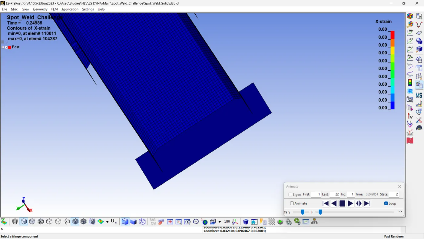
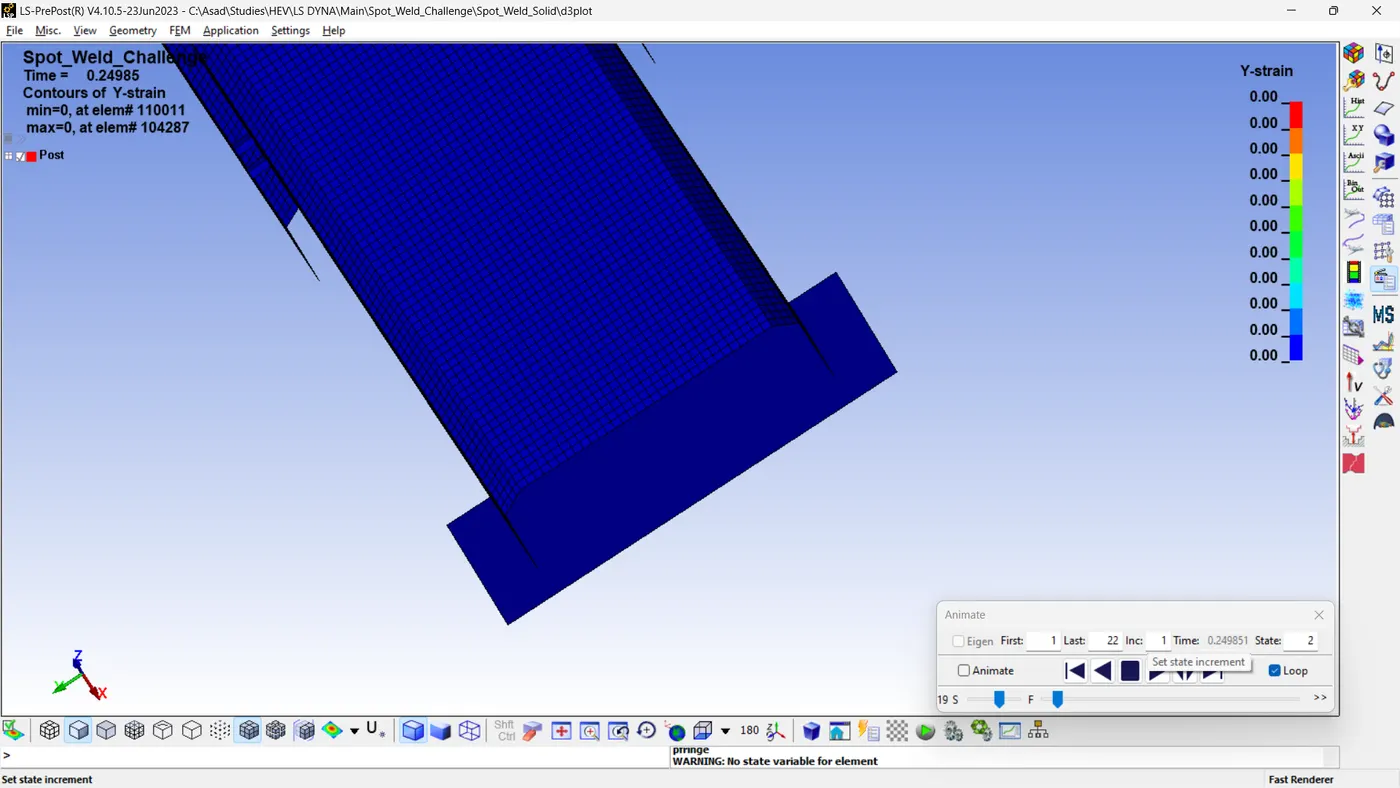
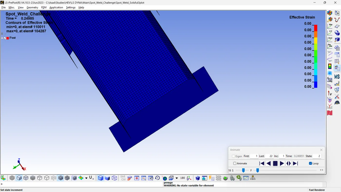
The simulation indicates that the X, Y and Von Mises strain values remain at zero.

3. Global Energies

The various energy plots and their observations are mentioned below.

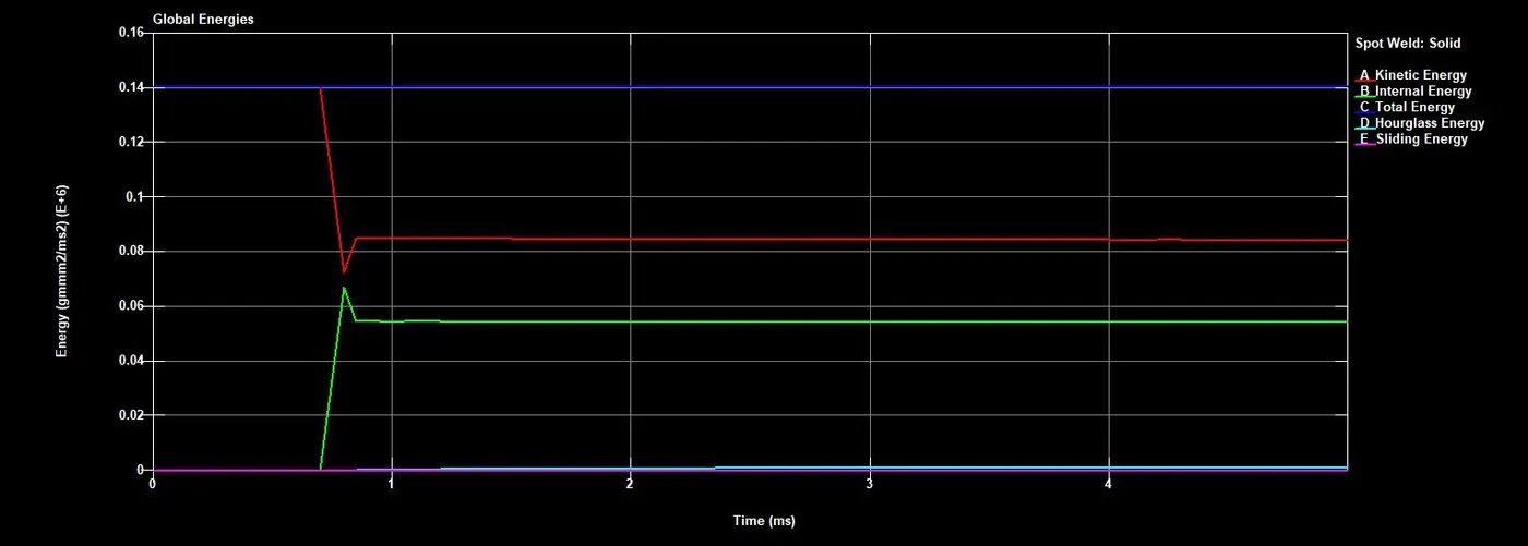
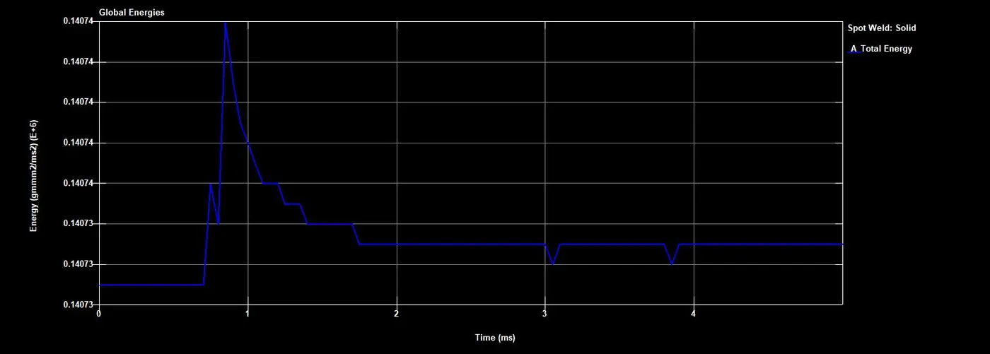
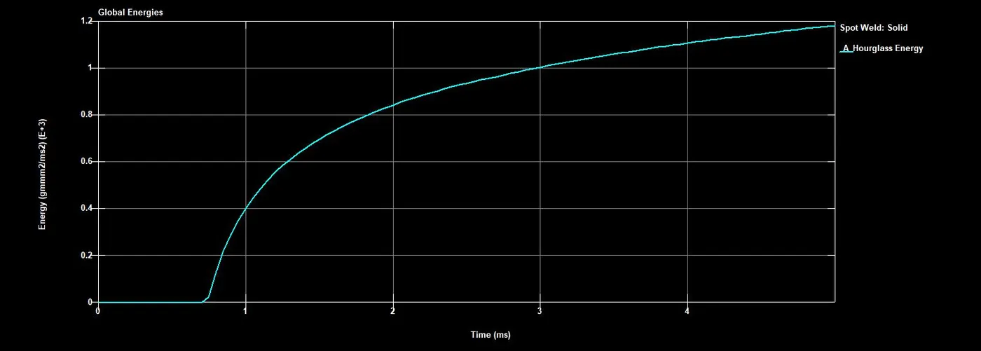
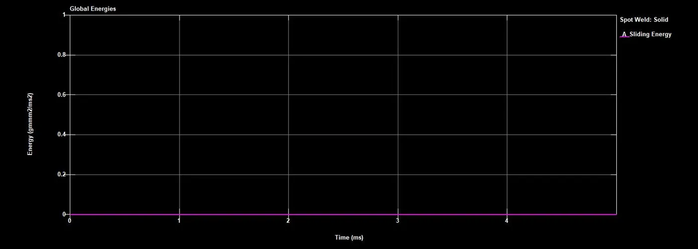
• As like model A, model B starts with KE of the maximum value of 1.40e5 within the first 0.699 seconds, which is attributable to the initial velocity of the model. Then the contact occurs, KE is converted to PE, so there is a rapid decrease in KE down to (7.29e4) due to this impact. Then it rebounds, and the velocity leads to a slight increase in kinetic energy (KE) to 8.53e4, which remains constant throughout the simulation.
  
  
• In the IE, the opposite of what occurs above takes place. The IE remains zero until the impact begins. At the time of the collision, the IE instantly increased its value to the maximum value (6.73e4) and The value then rapidly decreased to 5.47e4, which remains constant throughout the simulation.
  
  
• Unlike model A, these plots do not intersect, indicating that no deformation occurs.
  
  
• The entire crash's Total Energy (TE) initiates at 1.41e5. As the crash commences, followed by a gradual decline.
• Hourglass energy (HE) is not produced until the onset of the crash. The impact initiates the HE and gradually increases the value (more of a parabolic increase) (1.88e3) until the end of the simulation.
• The sliding energy is zero, indicating that no sliding or friction occurs.
  
  

4. Cross-Sectional Force
The sectional force for the mid-section of the crash box is illustrated below.

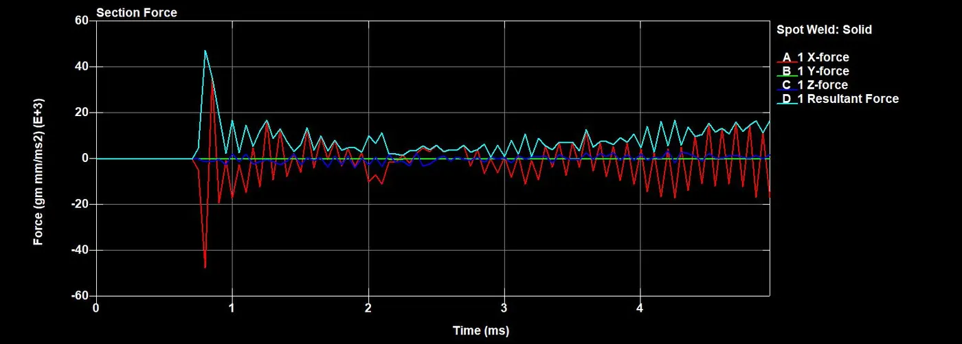
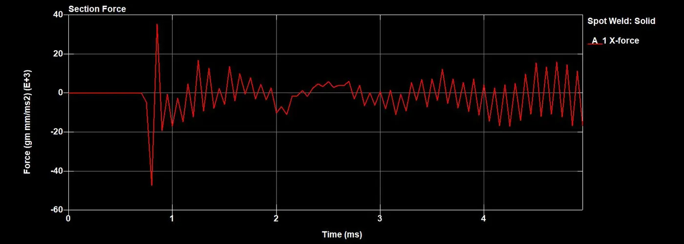
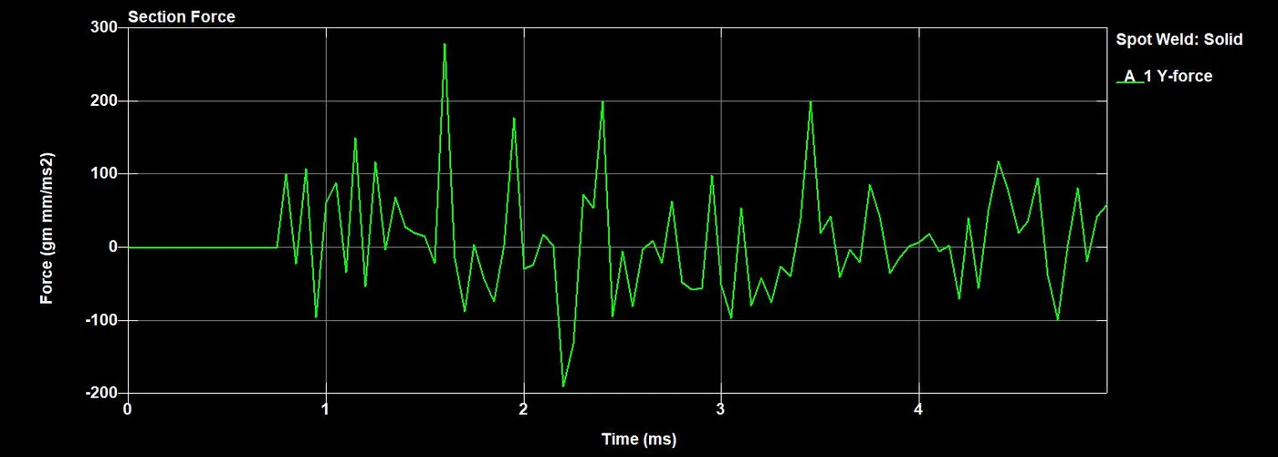
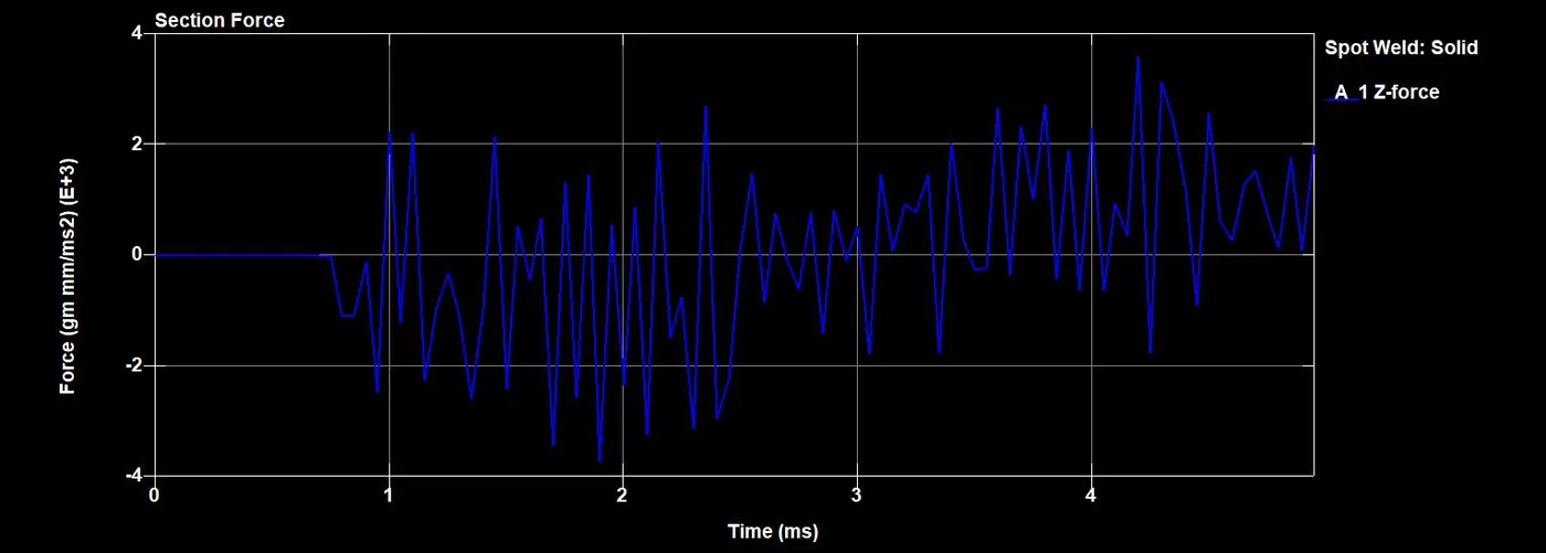
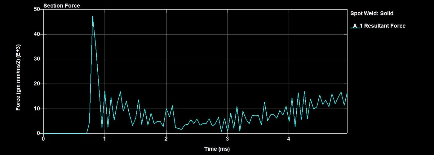
• The cross-sectional force in the x-direction is significantly higher than the forces on the y and z axes. The resultant forces remain at zero until the impact occurs. At the moment of impact, they spike sharply (4.73e4) before declining abruptly and fluctuating continuously.

5. Nodal Accelerations

The nodal accelerations for the mid-section of node ID 502639 in the crash box are illustrated below.

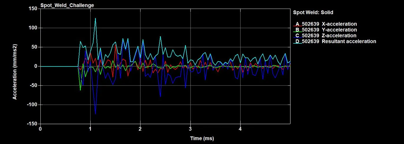
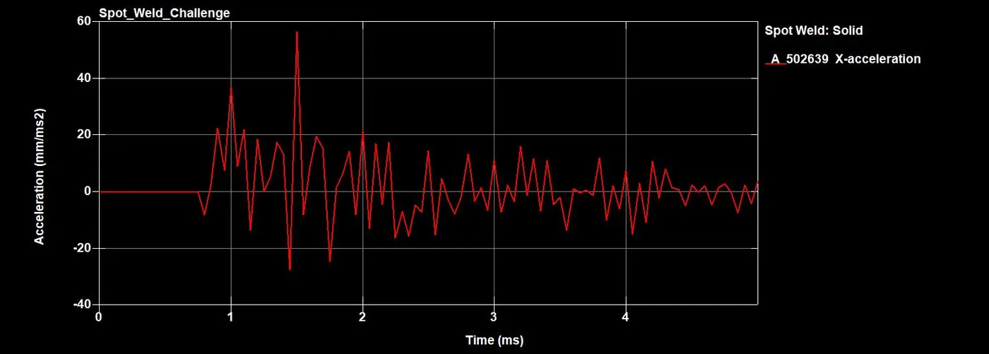
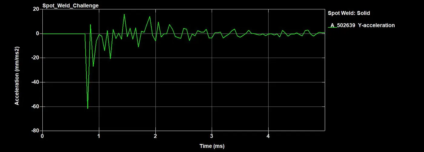
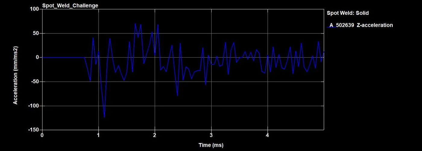
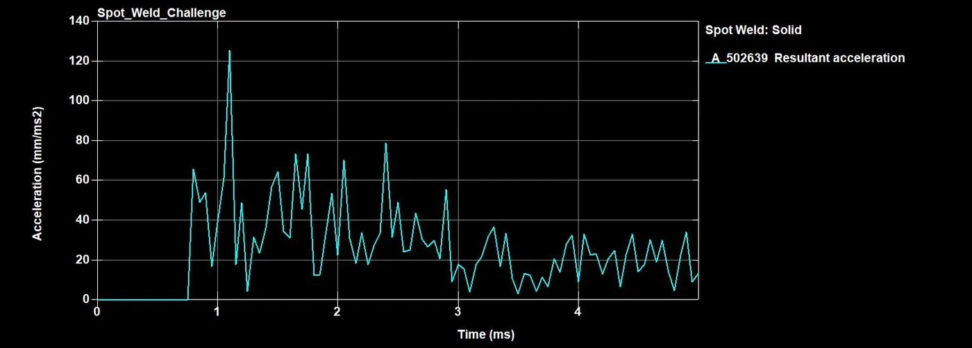
• The nodal accelerations in the x-direction are significantly higher than on the y and z axes. The resultant accelerations stay at zero until the impact takes place. The resultant accelerations stay at zero until the impact takes place. There is a sharp spike to approximately 65.8mm/ms2 at the instant of impact, followed by a sudden decline and continuous fluctuations. The peak acceleration happens almost instantly at about 1.10 ms, reaching up to 126 mm/ms².

Conclusion

• The simulation has been conducted for both scenarios, and the desired outcomes have been achieved.
• The analysis of stress and strain in both scenarios is facilitated by animations using d3plot.
• The analysis of cross-sectional forces and global energies has been completed, utilizing the plots for a comprehensive examination.
• The acceleration of the node (NID = 502639) is analyzed using plots for both scenarios.

Reference

• https://www.theworldmaterial.com/astm-a36-steel/

Drive Link: https://drive.google.com/file/d/1nf9mujKwmmso3snz-wgSLbOjEBq6h_MK/view?usp=sharing