Week 5 - Mid term project - Solving the steady and unsteady 2D heat conduction problem

Steady-state analysis & Transient State Analysis:

Solving the 2D heat conduction equation by using the point iterative techniques:
The Boundary conditions for the problem are as follows:
Top Boundary = 600 K
Bottom Boundary = 900 K
Left Boundary = 400 K
Right Boundary = 800 K
We will implement Jacobi, Gauss-seidel, Successive over-relaxation methods for solving implicit equations:

Assume Error fro accurate solution is (9e9)
Your absolute error criteria are 1e-4 (tolerance)

Heat transfer is the transfer of thermal energy from the body of higher temperature to another body at a lower temperature when both are in physical contact with each other. The heat transfer may occur under steady or unsteady state conditions.
In the steady-state conditions, the temperature within the system does not change with respect to time.
In Unsteady state conditions the temperature within the system change with respect to time. Unsteady state conditions are the precursor to the steady-state condition. No system exists initially under steady-state conditions. After heat transfer is initiated some time must pass before the system reaches steady-state. During the period of transition, the system is under an unsteady state condition, therefore, also called Transient state condition.
No system can remain in a steady-state condition perpetually. The temperature of the system will eventually reach the temperature of the heat source and once this occurs the system will be steady-state. Even if the amount of heat transferred to the system is increased, at some point the system reaches its critical temperature and the energy transferred into the system starts causing phase change within the system rather than temperature rise.

Steady-state heat conduction:

On solving steady-state heat conduction, we consider that there is no convection or internal heat generation in this problem. Thus the temperature of the body does not change with time and the heat conduction is a function of position only.

So, the general equation is given by:

`(∂^2T)/(∂x^2) + (∂^2T)/(∂y^2) = 0`

We use Numerical Method and the solution is obtained at discrete points in the unit square domain (like 10*10 or 20*20 0r 30*30). We start with mesh and describe our profile within the domain at discrete intervals. The spacing between the two discrete points in the x and y planer is (dx) and (dy) respectively. And the grid points (nx=ny). Now we formulate the general equation in such a way that we can set it up in a computer program. The steady-state equation can be solved only by explicit method, cause there is no time term in the governing equation.

On differentiating each term of the general equation is given by,

`(∂^2T)/(∂x^2) = (T(i+i,j) - 2T(i,j) + T(i-1,j))/(Δx^2)`

`(∂^2T)/(∂y^2) = (T(i,j-1) - 2T(i,j) + T(i,j+1))/(Δy^2)`

Summing up the equation, we get

`(∂^2T)/(∂x^2) + (∂^2T)/(∂y^2) = ((T(i+i,j) - 2T(i,j) + T(i-1,j))/(Δx^2)) + ((T(i,j-1) - 2T(i,j) + T(i,j+1))/(Δy^2))=0`

On the left had side:

((T(i+i,j) - 2T(i,j) + T(i-1,j))/(Δx^2)) + ((T(i,j-1) - 2T(i,j) + T(i,j+1))/(Δy^2))=0

On the L.H.S, taking out (2T(i,j)/Δx^2) and (2T(i,j)/Δy^2) common out, we get our final equation:

`((2*T(i,j))/(Δx^2))+((2*T(i,j))/(Δy^2)) = ((T(i+i,j) + T(i-1,j))/(Δx^2)) + ((T(i,j-1) + T(i,j+1))/(Δy^2))`

Further simpilification:

`T(i,j)((2*(Δx^2 +Δy^2))/(Δx^2*Δy^2)) = ((T(i+i,j) + T(i-1,j))/(Δx^2)) + ((T(i,j-1) + T(i,j+1))/(Δy^2))`

Let's consider the constants for simpler calculation:

`k =(2*(Δx^2+Δy^2))/(Δx^2*Δy^2)`

Substituting k1 and k2 on the final equation:

`T(i,j) = (k^-1)(((T(i+i,j) + T(i-1,j))/(Δx^2)) + ((T(i,j-1) + T(i,j+1))/(Δy^2)))`

From the above equation we can find the required temperature and the matlab program can be written using the same equation.

Matlab Code:

clear all 
close all 
clc

%Input parameters
L = 1;
nx = 30;
ny = 30;
%Domain is a unit square along x and y
x = linspace (0,L,nx);
y = linspace (0,L,ny);

%calculating the grid space
dx = L/(nx-1);
dy = L/(ny-1);

%Defining the constant K
k = (2*(dx^2+dy^2))/((dx^2)*(dy^2));

%Error and Tolerance
error = 9e9;
tol = 1e-4;

%Initial temperature 
T = ones(nx,ny);

%Temperature at Boundary line (units iun Kelvin(K))
T(2:ny-1,1) = 400; %Left 
T(2:ny-1,nx) = 800; %Right 
T(1,2:nx-1) = 600; %Top 
T(ny,2:nx-1) = 900; %Bottom 

%Temperature at the Corner
T(1,1) = (600+400)/2;
T(nx,ny) = (800+900)/2;
T(1,ny) = (600+800)/2;
T(nx,1) = (400+900)/2;

%Initializing the boundary condition
T_old = T;
T_initial = T;

%Choosing the solver
iterative_solver = input('1 for Jacobi, 2 for Gauss Seidel, 3 for SOR Enter the type of solver you would like to use: n =');

%jacobi iteration
tic
if iterative_solver==1
j_iteration=1;
[X,Y] = meshgrid(x,y);
while(error > tol)
    for i=2:nx-1
        for j=2:ny-1
            term_1 = (T_old(i-1,j)+T_old(i+1,j))/(dx^2);
            term_2 = (T_old(i,j-1)+T_old(i,j+1))/(dy^2);
            T(i,j) = (k^-1)*(term_1+term_2);
        end
    end
    error = max(max(abs(T_old-T)));
    T_old = T;
    j_iteration = j_iteration+1;
    
toc
jacobi_Time_val=toc;

%plotting
figure(1);
[P,Q] = contourf(X,Y,T);
clabel(P,Q);
colormap(jet);
colorbar;
title_text = sprintf('jacobi method, iteration number = %d, Time=%f s', j_iteration, jacobi_Time_val);
title(title_text)
xlabel ('Xaxis');
ylabel ('Yaxis');
set(gca,'Ydir','reverse')
pause(0.003);
end
end


%Gauss Seidel iteration
if iterative_solver ==2
tic
gs_iteration=1;
[X,Y] = meshgrid(x,y);
while(error > tol)
    for i=2:nx-1
        for j=2:ny-1
            term_1 = (T(i-1,j)+T_old(i+1,j))/(dx^2);
            term_2 = (T(i,j-1)+T_old(i,j+1))/(dy^2);
            T(i,j) = (k^-1)*(term_1+term_2);
        end
    end
    error = max(max(abs(T_old-T)));
    T_old = T;
    gs_iteration = gs_iteration+1;
    
toc
gauss_Time_val=toc;

%plotting
figure(1);
[A,B] = contourf(X,Y,T);
clabel(A,B);
colormap(jet);
colorbar;
title_text = sprintf('Gauss Seidel method, Iteration number = %d, Time=%f s', gs_iteration, gauss_Time_val);
title(title_text)
xlabel ('Xaxis');
ylabel ('Yaxis');
set(gca,'Ydir','reverse')
pause(0.03);
end
end


%SOR iteration
if iterative_solver==3
[X,Y] = meshgrid(x,y);
tic
sor_iteration=0;
w=1.2;
while(error > tol)
    for i=2:nx-1
        for j=2:ny-1
            term_1 = (T(i-1,j)+T_old(i+1,j))/(dx^2);
            term_2 = (T(i,j-1)+T_old(i,j+1))/(dy^2);
            T(i,j) = (1-w)*T_old(i,j)+(w*(k^-1)*(term_1+term_2));
        end
    end
    error = max(max(abs(T_old-T)));
    T_old = T;
    sor_iteration = sor_iteration+1;
    
toc
sor_Time_val=toc;

%plotting
figure(1);
[A,B] = contourf(X,Y,T);
clabel(A,B);
colormap(jet);
colorbar;
title_text = sprintf('SOR method, Iteration number = %d, Time=%f s', sor_iteration, sor_Time_val);
title(title_text)
xlabel ('Xaxis');
set(gca,'Ydir','reverse')
ylabel ('Yaxis');
pause(0.03);
end
end

Graph output:

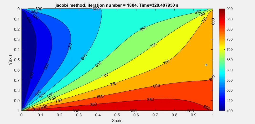
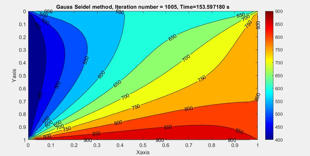
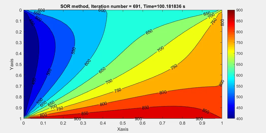
Description	Jacobi method	Gauss-Seidel method	SOR method
Iteration	1884	1005	691
Time in sec	320.40	153.59	100.18

From the data, we can clearly see that the SOR method has converged to the required tolerance of less than 1e-4 with a minimum number of iteration followed by Gauss_Seidel and the Jacobi methods. It makes sense, cause the Jacobi method didn't update the temperature value, and gauss_seidel does re-enter the latest temperature value in the calculation for better accuracy and to converge faster. And, SOR is literally scaling up by multiplying a relaxation factor `omega` to the gauss_seidal method. Thus it converges even faster than the gauss-seidel method, the optimal value of relaxation, omega `ω = 2/ (1+sin(πdx))`

And in Steady-state the are no time criteria, hence, there is no time marching approach, the temperature gradient remains the same throughout the simulation. Unlike the Unsteady-state equation, the Steady-state equation can be solved only by the Implicit method. The choice of the iteration methods highly depends upon the differential equation and boundary condition.

Transient State Heat Conduction:

In Transient state or Unsteady Heat Conduction, The temperature of the body varies with respect to both time and position either it is a one-dimensional or multi-1dimensional system. We assume there is no convection and no Internal Heat generation. The Governing Equation for 2D Transient heat conduction is given by

`(∂T)/(∂t) = α.((∂^2T)/(∂x^2)+(∂^2T)/(∂y^2))`

where t is the time in seconds and `α` is the temperature diffusivity of the material.
In the Method of characteristics, we learn that when having a time derivative in the governing equation we make use of the Time Marching approach. The solution is implemented by making use of numerical schemes at every discrete point on the square domain.
Rather not like steady-state equation the unsteady state equation can be solved by two methods Implicite method and the Explicite method

Solving the Unsteady State Equation using Explicit Method:

In this method, the governing differential equation is first discretized using any of the discretization methods, based on the Level of Accuracy required is the Order of Derivative required. After discretized the value of each node is evaluated until the desired node is reached. The method uses a time marching approach to solve the equation. So the nth step information is used to calculate the next step. The explicit method is the simplest method yet less accurate to solve the differential equation. In this equation, the time term is discretized using forward differencing and the space terms are discretized using central differencing.

Discretizing time term:

`(∂T_i,_j)/(∂t) =(( T_(i,j)^(n+1) - T_(i,j)^(n)))/(Δt)`

Discretizing space terms:

`(∂^2T_(i,j)^(n))/(∂x^2) = ((T_(i-i,j)^(n) - 2T_(i,j) ^(n)+ T_(i+1,j)^(n))/(Δx^2))`

`(∂^2T_(i,j)^(n))/(∂y^2) = ((T_(i,j-1)^(n) - 2T_(i,j)^(n) + T_(i,j+1)^(n))/(Δy^2))`

where i and j are the nodes in the 2D plane and n is the time counter.

Substituting the discretized terms in the general equation:

`(( T_(i,j)^(n+1) - T_(i,j)^(n)))/(Δt) = α*(((T_(i-i,j)^(n) - 2T_(i,j) ^(n)+ T_(i+1,j)^(n))/(Δx^2)) + ((T_(i,j-1)^(n) - 2T_(i,j)^(n) + T_(i,j+1)^(n))/(Δy^2)))`

Let us consider some constant for the simpler calculation k1 and k2

`k1 = ((α*Δt)/(Δx^2))`

`k2 = ((α*Δt)/(Δy^2))`

So the equation boils down to:

`( T_(i,j)^(n+1) - T_(i,j)^(n))= (k1*(T_(i-i,j)^(n) - 2T_(i,j) ^(n)+ T_(i+1,j)^(n)) )+ (k2*(T_(i,j-1)^(n) - 2T_(i,j)^(n) + T_(i,j+1)^(n)))`

`T_(i,j)^(n+1) = (T_(i,j)^(n)) + (k1*(T_(i-i,j)^(n) - 2T_(i,j) ^(n)+ T_(i+1,j)^(n)) )+ (k2*(T_(i,j-1)^(n) - 2T_(i,j)^(n) + T_(i,j+1)^(n)))`

Due to some stability reasons, we assume the CFL constant is 0.5.
CFL condition: It says the distance that any information travels during the timestep length with-in the mesh must be lower than the distance between the mesh element.
So the alpha is calculated accordingly to reach the constant. If CFL is above 0.5 the solution became Unstable.

Matlab Code:

clear all 
close all 
clc

%Input parameters
L = 1;
nx = 31;
ny = 31;

%Domain is a unit square along x and y
x = linspace (0,L,nx);
y = linspace (0,L,ny);
dx = L/(nx-1);
dy = L/(ny-1);

%Error and Tolerance
error = 1;
tol = 1e-4;

%Initial temperature 
T = ones(nx,ny);

%Temperature at Boundary line (units iun Kelvin(K))
T(2:ny-1,1) = 400; %Left (T_L)
T(2:ny-1,nx) = 800; %Right (T_R)
T(1,2:nx-1) = 600; %Top (T_T)
T(ny,2:nx-1) = 900; %Bottom (T_B)

%Temperature at the Corner
T(1,1) = (600+400)/2;
T(nx,ny) = (800+900)/2;
T(1,ny) = (600+800)/2;
T(nx,1) = (400+900)/2;

%Creating a copy of T
[X,Y] = meshgrid(x,y);

%Initializing the boundary condition
T_old = T;
T_initial = T;

%Input parameters for the equation:
alpha = 1.4; % Theremal Diffusivity
dt = dx^2/(4*alpha); %time step

%CFL Condition
k1 = (alpha*dt)/(dx^2);
k2 = (alpha*dt)/(dy^2);
CFL = k1+k2;

%time
t_start = 0;
t_end = 1;
%Simulation Parameters:
t = t_start:dt:t_end;
nt = length(t);

tic
unsteady_exp = 1;
for z = 1:nt
while(error > tol)
    for i=2:nx-1
        for j=2:ny-1
            t1 = T_old(i,j);
            t2 = T_old(i-1,j)-2*T_old(i,j)+T_old(i+1,j);
            t3 = T_old(i,j-1)-2*T_old(i,j)+T_old(i,j+1);
            T(i,j)= t1 + (k1*t2) +( k2*t3);
        end
    end
    error = max(max(abs(T_old-T)));
    T_old = T;
    unsteady_exp = unsteady_exp+1;
    
toc
exp_Timer_val=toc;


figure(1);
[A,B] = contourf(X,Y,T);
clabel(A,B);
colorbar;
colormap(jet);
xlabel ('Xaxis','FontSize',14');
ylabel ('Yaxis', 'FontSize',14);
set(gca,'Ydir','reverse')
str = {['Temperature contour at t =', num2str(t_end), 'Number of iteration =',num2str(unsteady_exp), 'using explicit scheme takes', num2str(exp_Timer_val),'s']};
text = ['Transient_analysis_','.png'];
title(str, 'FontSize',11)
pause (0.03)
fprintf('CFL number %f', CFL);

end
end

Graph:

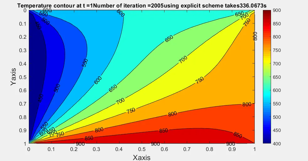
If we observe the data from the graph we can see that the explicit method has a more iteration compare to the Steady-state method, this is because of the addition of time derivative in the governing equation which increases the no of time steps in the Equation. The important thing about the explicit method is that it has stability criteria above which the solution blows up and that output can't be trustworthy. Thus the CFL condition is calculated and for a stable solution, the CFL value needs to be equal to or less than 0.5 for the solution to be stable.

Solving the Unsteady State Equation using Implicit Method:

The main difference between the Explicit method and the Implicit method is that the quantity to be evaluated at the current node takes the information from the current node rather than the previous node as seen in the Explicit method.

So, The general Equation is discretized as follows:

Discretizing time term:

`(∂T_i,_j)/(∂t) =(( T_(i,j)^(n+1) - T_(i,j)^(n)))/(Δt)`

Discretizing space terms:

`(∂^2T_(i,j)^(n+1))/(∂x^2) = ((T_(i-i,j)^(n+1) - 2T_(i,j) ^(n+1)+ T_(i+1,j)^(n+1))/(Δx^2))`

`(∂^2T_(i,j)^(n+1))/(∂y^2) = ((T_(i,j-1)^(n+1) - 2T_(i,j)^(n+1) + T_(i,j+1)^(n+1))/(Δy^2))`

where i and j are the nodes in the 2D plane and n is the time counter.

Let us consider some constant for the simpler calculation k1 and k2:

`k1 = ((α*Δt)/(Δx^2))`

`k2 = ((α*Δt)/(Δy^2))`

Substituting k1 and k2, we gat

`( T_(i,j)^(n+1) - T_(i,j)^(n))= (k1*(T_(i-i,j)^(n+1) - 2T_(i,j) ^(n+1)+ T_(i+1,j)^(n+1)) )+ (k2*(T_(i,j-1)^(n+1) - 2T_(i,j)^(n+1) + T_(i,j+1)^(n+1)))`

`( T_(i,j)^(n+1) - T_(i,j)^(n))= ((k1*T_(i-i,j)^(n+1) - k1*2T_(i,j) ^(n+1)+ k1*T_(i+1,j)^(n+1)) )+ ((k2*T_(i,j-1)^(n+1) -k2* 2T_(i,j)^(n+1) + k2*T_(i,j+1)^(n+1)))`

So, Rearranging the equation for `T_(i-i,j)^(n+1)` on one side, we get

`[T_(i,j)^(n+1) + ( k1*2T_(i,j) ^(n+1)) + (k2* 2T_(i,j)^(n+1)) ]= T_(i,j)^(n) + ((k1*T_(i-i,j)^(n+1) + k1*T_(i+1,j)^(n+1)) )+ ((k2*T_(i,j-1)^(n+1) + k2*T_(i,j+1)^(n+1)))`

`T_(i,j)^(n+1) (1+ (2*k1) + (2*k2) )= T_(i,j)^(n) + (k1*(T_(i-i,j)^(n+1) + T_(i+1,j)^(n+1)))+ (k2*(T_(i,j-1)^(n+1) + T_(i,j+1)^(n+1)))`

The Final Equation can be written as below:

`T_(i,j)^(n+1) =(1/(1+ (2*k1) + (2*k2) )) [T_(i,j)^(n) + (k1*(T_(i-i,j)^(n+1) + T_(i+1,j)^(n+1)))+ (k2*(T_(i,j-1)^(n+1) + T_(i,j+1)^(n+1)))]`

Matlab code:

clear all 
close all 
clc

%Input parameters
L = 1;
nx = 31;
ny = 31;

%Domain is a unit square along x and y
x = linspace (0,L,nx);
y = linspace (0,L,ny);
dx = L/(nx-1);
dy = L/(ny-1);

%Input parameters for the equation:
alpha = 0.047562; % Theremal Diffusivity
nt = 2000;
dt = 50;
k1 = (alpha*dt)/(dx^2);
k2 = (alpha*dt)/(dy^2);

%Error and Tolerance
error = 9e9;
tol = 1e-4;

%Initial temperature 
T = ones(nx,ny);

%Temperature at Boundary line (units iun Kelvin(K))
T(2:ny-1,1) = 400; 
T(2:ny-1,nx) = 800; 
T(1,2:nx-1) = 600; 
T(ny,2:nx-1) = 900; 

%Temperature at the Corner
T(1,1) = (600+400)/2;
T(nx,ny) = (800+900)/2;
T(1,ny) = (600+800)/2;
T(nx,1) = (400+900)/2;

%Creating a copy of T
[X,Y] = meshgrid(x,y);

%Initializing the boundary condition
T_old = T;
T_initial = T;
%calling the function
[T,error] = jacobi_unsteady_implitwo(T_old,T,x,y,nx,ny,error,k1,k2,tol);
[T,error] = gauss_unsteady_implicit (T_old,T,x,y,nx,ny,error,k1,k2,tol);
[T,error] = sor_unsteady_implicit (T_old,T,x,y,nx,ny,k1,k2,error,tol);

Functions:

Jacobi Method

%iterative solver using gauss Jacobi method
function [T,error] = jacobi_unsteady_implitwo(T_old,T,x,y,nx,ny,error,k1,k2,tol)
[X,Y] = meshgrid(x,y);
CFL = k1+k2;
%T_old = T;
T_initial = T_old;
tic
jacobi_iteration=0;
while (error>tol)
for i = 2:nx-1
    for j = 2:ny-1
        t1 = (1+(2*k1)+(2*k2))^-1;
        t2 = (T_old(i-1,j)+T_old(i+1,j));
        t3 = (T_old(i,j-1)+T_old(i,j+1));
        T(i,j) = t1*((T_initial(i,j))+(k1*t2)+(k2*t3));
    end
end
        error = max(max(abs(T_old-T)));
        T_old = T;
        jacobi_iteration = jacobi_iteration+1;
        jacobi_timer = toc;
        
        
figure(1)
[P,Q] = contourf(X,Y,T);
clabel(P,Q);
colormap(jet);
colorbar;
title (sprintf('2D Heat conduction implicit method, No.of jacobi iteration = %d,computation time = %fs', jacobi_iteration,jacobi_timer));
xlabel ('Xaxis')
ylabel ('Yaxis')
set(gca,'Ydir','reverse')
fprintf('Counter=%d,Time=%fs,CFL=%d,error=%f\n',jacobi_iteration,jacobi_timer,CFL,error);
pause(0.03)

end
end

Gauss-Seidel method:

%iterative solver using gauss seidel method

function [T,error] = gauss_unsteady_implicit (T_old,T,x,y,nx,ny,error,k1,k2,tol)
[X,Y] = meshgrid(x,y);
CFL = k1+k2;
T_initial = T_old;
gauss_iter = 0;
tic
while (error>tol)
   for i = 2:nx-1
       for j = 2:ny-1
           t1 = (1+(2*k1)+(2*k2))^-1;
           t2 = T(i-1,j)+T_old(i+1,j);
           t3 = T(i,j-1)+T_old(i,j+1);
           T(i,j) = t1*(T_initial(i,j)+(k1*t2)+(k2*t3));
       end 
   end
    error = max(max(abs(T_old-T)));
    T_old = T;
    gauss_iter = gauss_iter +1;
    gauss_timer = toc;
    
    
figure(2)
[P,Q] = contourf(X,Y,T);
clabel(P,Q);
colormap(jet);
colorbar;
title (sprintf('2D Heat Conduction Equation Implicit method, No of gauss seidel iteration = %d,computation time = %fs',gauss_iter,gauss_timer));
xlabel ('Xaxis');
ylabel ('Yaxis');
set(gca,'Ydir','reverse');
fprintf ('Counter = %d, Time = %fs,CFL=%d, error=%f\n',gauss_iter, gauss_timer,CFL, error);
pause(0.03)

end
end

SOR Method:

%iterative solver using SOR method

function [T,error] = sor_unsteady_implicit (T_old,T,x,y,nx,ny,k1,k2,error,tol)
[X,Y] =meshgrid(x,y);
w=1.2;
CFL = k1+k2;
T_initial = T;
tic
sor_iteration = 0;
while error>tol
      for i=2:nx-1
      for j = 2:ny-1
          t1 = (1+(2*k1)+(2*k2))^-1;
           t2 = T(i-1,j)+T_old(i+1,j);
           t3 = T(i,j-1)+T_old(i,j+1);
           T(i,j) = t1*(T_initial(i,j)+(k1*t2)+(k2*t3));
           T(i,j) = ((1-w)*T_old(i,j))+(w*T(i,j));      
      end
      end
      error = max(max(abs(T-T_old)));
      T_old = T;
      sor_iteration = sor_iteration +1;
      
toc
sor_timer = toc;

figure(3)
[P,Q] = contourf(X,Y,T);
clabel(P,Q);
colormap(jet);
colorbar;
title (sprintf('2D Heat Conduction Equation Implicit method, No of SOR iteration = %d,computation time = %fs',sor_iteration,sor_timer));
xlabel ('Xaxis');
ylabel ('Yaxis');
set(gca,'Ydir','reverse');
fprintf ('Counter = %d, Time = %fs,CFL=%d error=%f\n',sor_iteration, sor_timer,CFL, error);
pause(0.03)
end
end

[Note]: Before RUN the program, function out the line of code that you don't need, I mean, function out Gauss-Seidel and SOR while solving the Jacobi method and vice versa.

Graph:

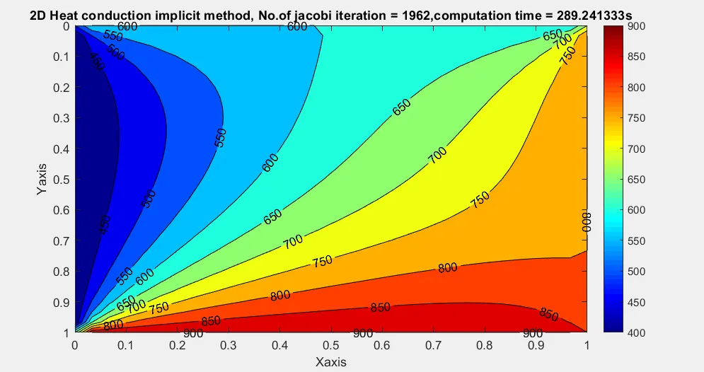
Jacobi method:

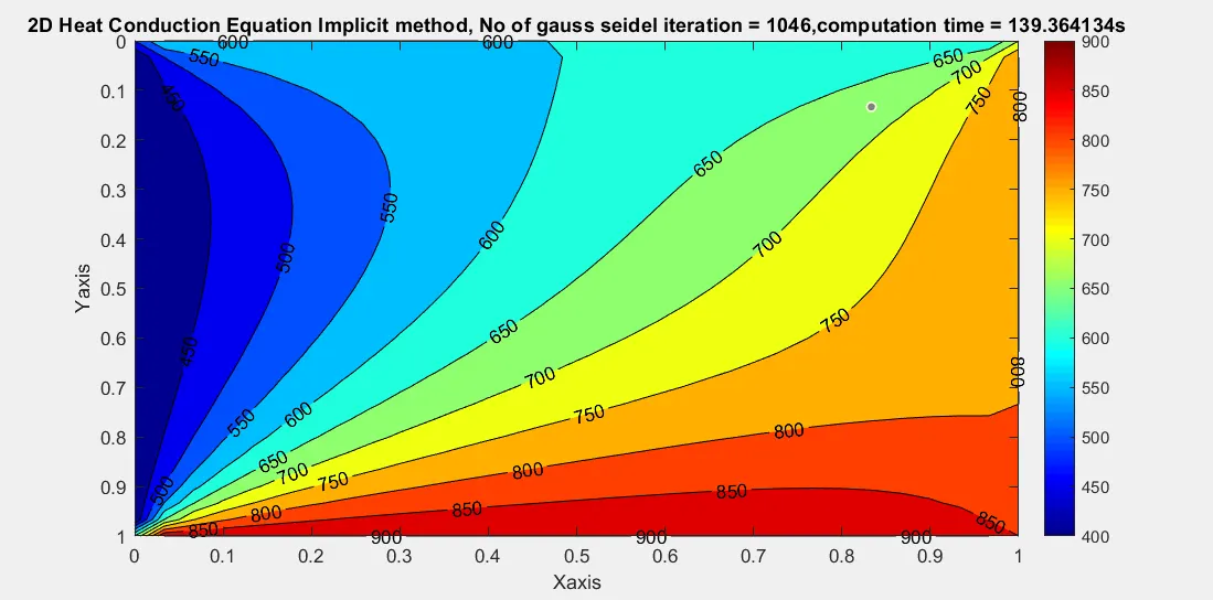
Gauss-Seidel method:

SOR method:

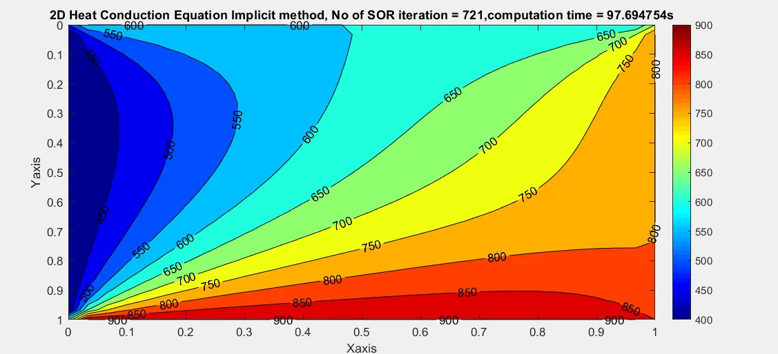
From the equation, u can see that the implicit method has the time marching solution, but the difference is that unconditionally stable (no stability criteria), so even higher CFL values can't affect the solution. From the graph, the data are tabulated below

Description	Jacobi method	Gauss-Seidel method	SOR method
Iteration	1962	1046	721
Time in sec	289.24	139.36	97.69

Here you can see the Transient implicit method takes the least amount of time for respective methods compared to steady-state methods. However, the same trend follows as the steady-state equation, the SOR method has converged to the required tolerance of less than 1e-4 with a minimum number of iteration followed by Gauss_Seidel and the Jacobi methods. It makes sense, cause the Jacobi method didn't update the temperature value, and gauss_seidel does re-enter the latest temperature value in the calculation for better accuracy and to converge faster. And, SOR is literally scaling up by multiplying an alpha parameter `alpha` to the gauss-seidel method. Thus it converges even faster than the gauss-seidel method, the optimal value of over-relaxation is 1.4.