Week 5 - Mid term project - Solving the steady and unsteady 2D heat conduction problem
Objective :- Solution of 2D steady and unsteady heat conduction problem .
Given Data :-
Boundary Conditions :-
1. Top Boundary =600 K
2. Bottom Boundary = 900 K
3. Left Boundary = 400 K
4. Right Boundary = 800 K
We will solve the problem by Jacobi method , Gauss -siedel method and Succesive Over relaxation method where absolute error criteria is 1e-4.
Steady State Analysis :- If the parameter to be measured is not a function of time then the analysis is said to be steady state analysis . For steady state analysis we are using the equation
`(d^2T)/dx^2+(d^2T)/dy^2=0`
Unsteady state analysis :- In case of fluid if the velocity of the fluid is a function of time or dependent on time then the analysis is said to be unsteady state analysis but in case of heat transfer we are dealing with temperature so if the temperature is dependent on time like in initial stages of analysis then the analyis is said to be transient analysis .So here we are dealing with transient analysis .
And for unsteady analysis we are using the equation :-
`alpha[(d^2T)/dx^2+(d^2T)/dy^2]=(dT)/(d tau)`.
Taking number of nodes on x axis equal to number of nodes along y axis makes `delta x=delta y` and discretization of equation becomes easy to handle .Using central differencing scheme for discretization we get :-
`(d^2T)/(dx^2)=(T(i-1,j)-2T(i,j)+T(i+1,j))/(deltax)^2`.
`(d^2T)/(dy^2)=(T(i,j-1)-2T(i,j)+T(i,j+1))/(deltay^2)`.
therefore on putting the values and solving the equation we get :-
`T(i,j)=1/4(T(i-1,j)+T(i+1,j)+T(i,j-1)+T(i,j+1))` where `deltax=deltay`
Matlab Code for steady and implicit method by using Jacobi Method
% Steady State Solution by using Jacobi method
close all
clear all
clc
% Input parameters
n_x=20;
n_y=n_x;

x=linspace(0,1,n_x);
y= linspace(0,1,n_y);
dx=x(2)-x(1);
dy=dx;
error = 9e9;
tolerance= 1e-4;
T_L = 400;
T_R = 800;
T_T = 600;
T_B = 900;
T=300 * ones (n_x,n_y);
T(2:n_y-1,1) = T_L;
T(2:n_y-1,n_x)= T_R;
T(1,2:n_x -1)= T_T;
T(n_y,2:n_x -1)= T_B;

% Calculation of average temperature at each corner
T(1,1)=(T_T+T_L)/2;
T(n_x,n_y)=(T_B+T_R)/2;
T(1,n_y)= (T_T+T_R)/2;
T(n_x,1)=(T_L+T_B)/2;

T_initial =T;
T_old=T;

iterative_solver=1;
if iterative_solver==1
    jacobi_iteration = 1;
    while (error>tolerance)
        for i =2:n_x-1
            for j=2:n_y-1
                T(i,j)= 0.25 *(T_old(i-1,j)+T_old(i+1,j)+T_old(i,j-1)+T_old(i,j+1));
            end
        end
        error = max(max(abs(T_old-T)));
        T_old=T;
        jacobi_iteration=jacobi_iteration+1;
    end
end
% Plotting the graph
figure (1)
contourf(x,y,T)
clabel(contourf(x,y,T))
colorbar
colormap(jet)
set(gca,'ydir','reverse')
xlabel('X-axis')
ylabel('Y-axis')
title(sprintf('No of Jacobi Iterations (Implicit)=%d',jacobi_iteration));
pause(0.03);
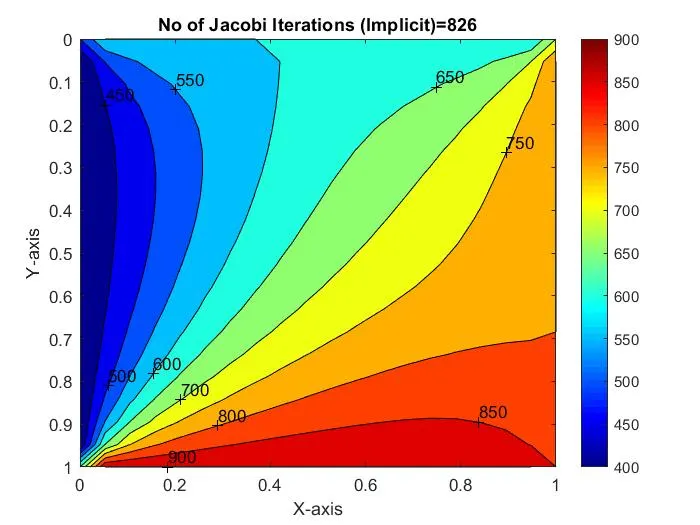
Output :-
Gauss -Siedel Method :-
Matlab Code
% Steady State Solution by using Gauss -Siedel method
close all
clear all
clc
% Input parameters
n_x=20;
n_y=n_x;

x=linspace(0,1,n_x);
y= linspace(0,1,n_y);

dx=x(2)-x(1);
dy=dx;
error = 9e9;
tolerance= 1e-4;
T_L = 400;
T_R = 800;
T_T = 600;
T_B = 900;
T=300 * ones (n_x,n_y);
T(2:n_y-1,1) = T_L;
T(2:n_y-1,n_x)= T_R;
T(1,2:n_x -1)= T_T;
T(n_y,2:n_x -1)= T_B;

% Calculation of average temperature at each corner
T(1,1)=(T_T+T_L)/2;
T(n_x,n_y)=(T_B+T_R)/2;
T(1,n_y)= (T_T+T_R)/2;
T(n_x,1)=(T_L+T_B)/2;

T_initial =T;
T_old=T;

iterative_solver=2;
if iterative_solver==2
    gauss_siedel_iteration = 1;
    while (error>tolerance)
        for i =2:n_x-1
            for j=2:n_y-1
                T(i,j)= 0.25 *(T(i-1,j)+T_old(i+1,j)+T(i,j-1)+T_old(i,j+1));
            end
        end
        error = max(max(abs(T_old-T)));
        T_old=T;
        gauss_siedel_iteration=gauss_siedel_iteration+1;
    end
end
% Plotting the graph
figure (1)
contourf(x,y,T)
clabel(contourf(x,y,T))
colorbar
colormap(jet)
set(gca,'ydir','reverse')
xlabel('X-axis')
ylabel('Y-axis')
title(sprintf('No of Gauss- Siedel-Iterations (Implicit)=%d',gauss_siedel_iteration));
pause(0.03);
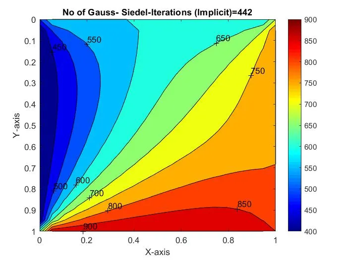
Output:-
Successive -over-relaxation method :-
Matlab Code:-
% Steady State Solution by using Gauss -Siedel method
close all
clear all
clc
% Input parameters
n_x=20;
n_y=n_x;
omega = 1.2;

x=linspace(0,1,n_x);
y= linspace(0,1,n_y);

dx=x(2)-x(1);
dy=dx;
error = 9e9;
tolerance= 1e-4;
T_L = 400;
T_R = 800;
T_T = 600;
T_B = 900;
T=300 * ones (n_x,n_y);
T(2:n_y-1,1) = T_L;
T(2:n_y-1,n_x)= T_R;
T(1,2:n_x -1)= T_T;
T(n_y,2:n_x -1)= T_B;

% Calculation of average temperature at each corner
T(1,1)=(T_T+T_L)/2;
T(n_x,n_y)=(T_B+T_R)/2;
T(1,n_y)= (T_T+T_R)/2;
T(n_x,1)=(T_L+T_B)/2;

T_initial =T;
T_old=T;

iterative_solver=3;
if iterative_solver==3
    Succesive_over_relaxation_iteration = 1;
    while (error>tolerance)
        for i =2:n_x-1
            for j=2:n_y-1
                T(i,j)= omega*(0.25 *(T(i-1,j)+T_old(i+1,j)+T(i,j-1)+T_old(i,j+1)))+(1-omega)*T_old(i,j);
            end
        end
        error = max(max(abs(T_old-T)));
        T_old=T;
        Succesive_over_relaxation_iteration=Succesive_over_relaxation_iteration+1;
    end
end
% Plotting the graph
figure (1)
contourf(x,y,T)
clabel(contourf(x,y,T))
colorbar
colormap(jet)
set(gca,'ydir','reverse')
xlabel('X-axis')
ylabel('Y-axis')
title(sprintf('No of Succesive over relaxation iterations (Implicit)=%d',Succesive_over_relaxation_iteration));
pause(0.03);
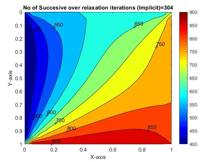
Output:-
Transient Analysis of 2D heat conduction equation :-
Matlab Code for Jacobi by Implicit Technique :-
% Unsteady State Solution by using Jacobi method (Implicit Technique)
close all
clear all
clc
% Input parameters
n_x=20;
n_y=n_x;
n_t=1400;
dt=1e-3;
alpha=1.1;

x=linspace(0,1,n_x);
y= linspace(0,1,n_y);
dx=x(2)-x(1);
dy=dx;
error = 9e9;
tolerance= 1e-4;
T_L = 400;
T_R = 800;
T_T = 600;
T_B = 900;
T=300 * ones (n_x,n_y);
T(2:n_y-1,1) = T_L;
T(2:n_y-1,n_x)= T_R;
T(1,2:n_x -1)= T_T;
T(n_y,2:n_x -1)= T_B;

% Calculation of average temperature at each corner
T(1,1)=(T_T+T_L)/2;
T(n_x,n_y)=(T_B+T_R)/2;
T(1,n_y)= (T_T+T_R)/2;
T(n_x,1)=(T_L+T_B)/2;

T_initial =T;
T_old=T;

%Calculation of K1 and K2
K1=alpha*(dt/(dx^2));
K2=alpha*(dt/(dy^2));

    jacobi_iteration = 1;
    for k=1:n_t
        error=9e9;

    while (error>tolerance)
        for i =2:n_x-1
            for j=2:n_y-1
                Term_1=1/(1+(2*K1)+(2*K2));
                Term_2 = K1*Term_1;
                Term_3 = K2*Term_1;
                H=(T_old(i-1,j))+(T_old(i+1,j));
                V=(T_old(i,j+1))+(T_old(i,j-1));

                T(i,j)= (T_initial(i,j)*Term_1)+(H*Term_2)+(V*Term_3);
            end
        end
        error = max(max(abs(T_old-T)));
        T_old=T;
        jacobi_iteration=jacobi_iteration+1;
    end
    T_initial=T;
% Plotting the graph
figure (1)
contourf(x,y,T)
clabel(contourf(x,y,T))
colorbar
colormap(jet)
set(gca,'ydir','reverse')
xlabel('X-axis')
ylabel('Y-axis')
title(sprintf('No of Unsteady Jacobi Iterations (Implicit)=%d',jacobi_iteration));
pause(0.03);
end
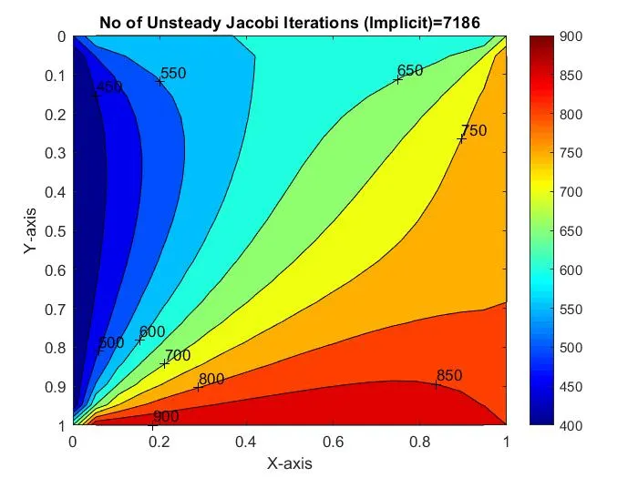
Output:-
Gauss Siedel Method for Unsteady state :-
Matlab Code:-
% Unsteady State Solution by using Gauss-Siedel- method (Implicit Technique)
close all
clear all
clc
% Input parameters
n_x=20;
n_y=n_x;
n_t=1400;
dt=1e-3;
alpha=1.1;

x=linspace(0,1,n_x);
y= linspace(0,1,n_y);
dx=x(2)-x(1);
dy=dx;
error = 9e9;
tolerance= 1e-4;
T_L = 400;
T_R = 800;
T_T = 600;
T_B = 900;
T=300 * ones (n_x,n_y);
T(2:n_y-1,1) = T_L;
T(2:n_y-1,n_x)= T_R;
T(1,2:n_x -1)= T_T;
T(n_y,2:n_x -1)= T_B;

% Calculation of average temperature at each corner
T(1,1)=(T_T+T_L)/2;
T(n_x,n_y)=(T_B+T_R)/2;
T(1,n_y)= (T_T+T_R)/2;
T(n_x,1)=(T_L+T_B)/2;

T_initial =T;
T_old=T;

%Calculation of K1 and K2
K1=alpha*(dt/(dx^2));
K2=alpha*(dt/(dy^2));

    gauss_siedel_iteration = 1;
    for k=1:n_t
        error=9e9;

    while (error>tolerance)
        for i =2:n_x-1
            for j=2:n_y-1
                Term_1=1/(1+(2*K1)+(2*K2));
                Term_2 = K1*Term_1;
                Term_3 = K2*Term_1;
                H=(T(i-1,j))+(T_old(i+1,j));
                V=(T(i,j+1))+(T_old(i,j-1));

                T(i,j)= (T_initial(i,j)*Term_1)+(H*Term_2)+(V*Term_3);
            end
        end
        error = max(max(abs(T_old-T)));
        T_old=T;
        gauss_siedel_iteration=gauss_siedel_iteration+1;
    end
    T_initial=T;
% Plotting the graph
figure (1)
contourf(x,y,T)
clabel(contourf(x,y,T))
colorbar
colormap(jet)
set(gca,'ydir','reverse')
xlabel('X-axis')
ylabel('Y-axis')
title(sprintf('No of Unsteady Gauss Siedel Iterations (Implicit)=%d',gauss_siedel_iteration));
pause(0.03);
    end
Output:-
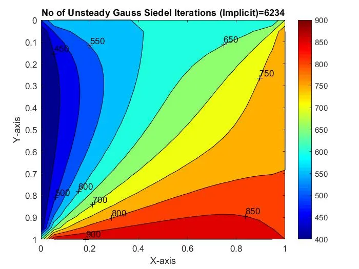
Transient Successive Over Relaxation (Implicit Technique) :-
% Unsteady State Solution by using Successive-Over-Relaxation-method (Implicit Technique)
close all
clear all
clc
% Input parameters
n_x=20;
n_y=n_x;
n_t=1400;
dt=1e-3;
alpha=1.1;
omega=1.2;

x=linspace(0,1,n_x);
y= linspace(0,1,n_y);
dx=x(2)-x(1);
dy=dx;
error = 9e9;
tolerance= 1e-4;
T_L = 400;
T_R = 800;
T_T = 600;
T_B = 900;
T=300 * ones (n_x,n_y);
T(2:n_y-1,1) = T_L;
T(2:n_y-1,n_x)= T_R;
T(1,2:n_x -1)= T_T;
T(n_y,2:n_x -1)= T_B;

% Calculation of average temperature at each corner
T(1,1)=(T_T+T_L)/2;
T(n_x,n_y)=(T_B+T_R)/2;
T(1,n_y)= (T_T+T_R)/2;
T(n_x,1)=(T_L+T_B)/2;

T_initial =T;
T_old=T;
T_end=T;

%Calculation of K1 and K2
K1=alpha*(dt/(dx^2));
K2=alpha*(dt/(dy^2));

    successive_over_relaxations_iteration = 1;
    for k=1:n_t
        error=9e9;

    while (error>tolerance)
        for i =2:n_x-1
            for j=2:n_y-1
                Term_1=1/(1+(2*K1)+(2*K2));
                Term_2 = K1*Term_1;
                Term_3 = K2*Term_1;
                H=(T(i-1,j))+(T_old(i+1,j));
                V=(T(i,j+1))+(T_old(i,j-1));

                T(i,j)= (T_initial(i,j)*Term_1)+(H*Term_2)+(V*Term_3);
                T_end (i,j) = (omega*T(i,j))+((1-omega)*T_old(i,j));
            end
        end
        error = max(max(abs(T_old-T)));
        T_old=T_end;
         successive_over_relaxations_iteration=successive_over_relaxations_iteration+1;
    end
    T_initial=T_end;
% Plotting the graph
figure (1)
contourf(x,y,T)
clabel(contourf(x,y,T))
colorbar
colormap(jet)
set(gca,'ydir','reverse')
xlabel('X-axis')
ylabel('Y-axis')
title(sprintf('No of successive over relaxations  Iterations (Implicit)=%d',successive_over_relaxations_iteration));
pause(0.03);
    end
Output :-
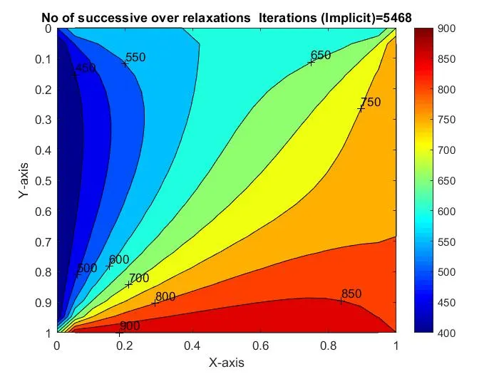
Unsteady State Analysis Using Explicit Technique:-
Matlab Code:-
% Unsteady State Solution by using  (Explicit Technique)
close all
clear all
clc
% Input parameters
n_x=20;
n_y=n_x;
n_t=1400;
dt=1e-3;
alpha=1.1;
omega=1.2;

x=linspace(0,1,n_x);
y= linspace(0,1,n_y);
dx=x(2)-x(1);
dy=dx;
error = 9e9;
tolerance= 1e-4;
T_L = 400;
T_R = 800;
T_T = 600;
T_B = 900;
T=300 * ones (n_x,n_y);
T(2:n_y-1,1) = T_L;
T(2:n_y-1,n_x)= T_R;
T(1,2:n_x -1)= T_T;
T(n_y,2:n_x -1)= T_B;

% Calculation of average temperature at each corner
T(1,1)=(T_T+T_L)/2;
T(n_x,n_y)=(T_B+T_R)/2;
T(1,n_y)= (T_T+T_R)/2;
T(n_x,1)=(T_L+T_B)/2;

T_initial = T;
T_old = T;

%Calculation of K1 and K2
iterative_solver = 6;
K1=alpha*(dt/(dx^2));
K2=alpha*(dt/(dy^2));

if iterative_solver == 6
    Unsteady_explicit = 1;

    for K=1:n_t
        error=9e9;

    while (error>tolerance)
        for i =2:n_x-1

            for j=2:n_y-1

                Term_1 = T_old(i,j);
                Term_2 = K1*(T_old(i+1,j)-2*T_old(i,j)+(T_old(i-1,j)));
                Term_3 = K2*(T_old(i,j+1)-2*T_old(i,j)+T_old(i,j-1));
                T(i,j)= Term_1+Term_2+Term_3;
            end
        end
        error = max(max(abs(T_old-T)));
        T_old=T;
        Unsteady_explicit = Unsteady_explicit + 1;
    end
    end
end
% Plotting the graph
figure (1)
contourf(x,y,T)
clabel(contourf(x,y,T))
colorbar
colormap(jet)
set(gca,'ydir','reverse')
xlabel('X-axis')
ylabel('Y-axis')
title(sprintf('No. of Unsteady Iterations (Explicit)=%d',Unsteady_explicit));
pause(0.03);
Output:-
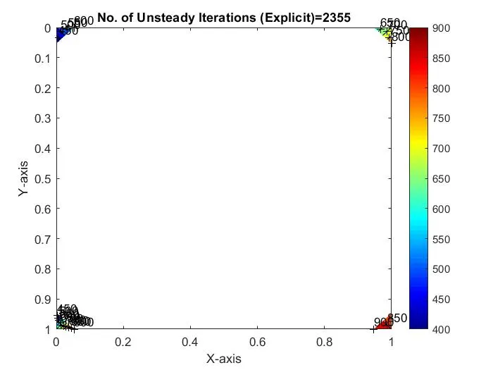
No of Unsteady Iterations = 2355
Conclusions
1. Jacobi>Gauss -Siedel>Successive Over Relaxation Method . In steady state analysis by implicit technique Jacobi takes the highest number of iterations and succesive over relaxation method takes the least number of iterations .
2. Among steady state and transient analysis , steady state analysis takes the least time for computation .
3. Successive Over Relaxation Method is the most effective method for steady state and transient analysis among both implicit and explicit technique .