Week 5 - Genetic Algorithm

Aim:

1. Explain the concept of Genetic Algorithm.
2. Explain the syntax for Genetic Algorithm in MATLAB.
3. Write a code to optimize the stalagmite function
4. Write a code to find the global maxima of the function.

Objectives of the project:

Write a code in MATLA to optimize the stalagmite function and find the global maxima of the function

What is Genetic Algorithm

Genetic Algorithm: Genetic Algorithm (GA) is a branch of field of study called evolutionary commutation. It is based on evolution theory by Darwin. GA is used to optimize a given function to find its maximum or minimum value. The basic components of a GA are

1. Fitness function: It is the function that GA is trying to optimize.
2. A population of chromosome: It is the numerical values that represent all the solutions to the function. The selection operator chooses some of the chromosomes (with replacement) for reproduction based on probability distribution. Fitter the chromosome more likely it is to be selected.
3. Cross over: This operator swaps in random a subsequence of two of the chosen chromosomes to create two offspring. Usually each chromosome is converted into binary code and then cross over is done from one parent chromosome into another.
4. Mutation: Mutation operator randomly flips individual bits in the new chromosomes.

GA Syntax

1.x = ga(fun,nvars) finds a local unconstrained minimum, x, to the objective function, fun. nvars is the dimension (number of design variables) of fun.

2. x = ga(fun,nvars,A,b,Aeq,beq,lb,ub,nonlcon,intcon,options)

fun = objective function

nvars = number of variables

A and B = subject to linear inequalities of the form A*x <=B

Aeq and Beq = subject to linear equalities of the form A*x = B

LB = lower bound

UB = upper bound

nonlcon = non linear inequalities

intcon = integer constrained

options = helps to add contraint tolerance by increasing the population size

Body of the content:

Incase of programming project

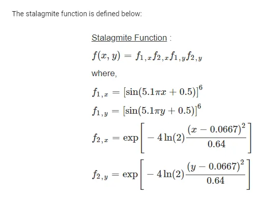
Code for stalagmite Function:

function [f] = stalgmite(input_vector)
x = input_vector(1);
y = input_vector(2);

f1_x =(sin((5.1*pi*x)+0.5)).^6;
f1_y =(sin((5.1*pi*y)+0.5)).^6;

f2_x = exp(((-4*log(2))*(x-0.0667).^2)/0.64);
f2_y = exp(((-4*log(2))*(y-0.0667).^2)/0.64);

[f] = -(f1_x.*f1_y.*f2_x.*f2_y);
end

Main Program:

clear
close
clc

% Defining our search space
x = linspace(0,0.6,150);
y = linspace(0,0.6,150);

% Creating a 2D mesh

[xx yy] = meshgrid(x,y);

Num_case =80;

% Evaluating a stalgmite function

for i =1:length(xx)
    for j=1:length(yy)
        input_vector(1)=xx(i,j);
        input_vector(2)=yy(i,j);
        f(i,j)=stalgmite(input_vector);
    end
end





% Study 1 - static behavior

tic
for i=1:Num_case
    [inputs,fopt(i)]=ga(@stalgmite,2);
    xopt(i)=inputs(1);
    yopt(i)=inputs(2);

end


study1_time=toc;

figure(1)
subplot(2,1,1)
hold on
surfc(xx,yy,-f)
shading interp
title('unbound inputs')
xlabel('X values')
ylabel('Y values')
plot3(xopt,yopt,-fopt,'marker','o','markersize',5,'markerfacecolor','r')


subplot (2,1,2)
plot(-fopt)  
xlabel('iterations')
ylabel('function maxima')

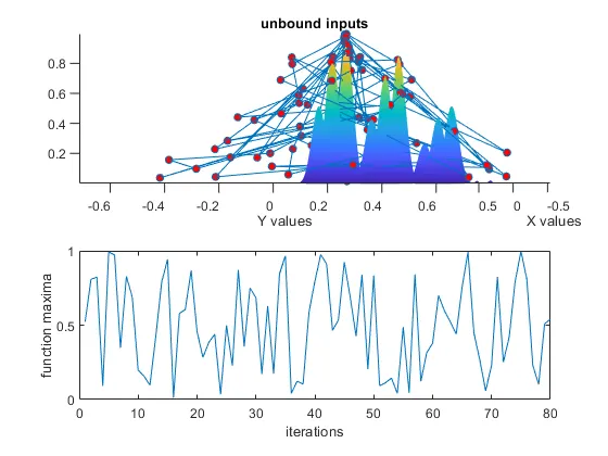
Plot of unbounded inputs:

% Study 2 - statistical behaviour with upper and lower bounds

tic
for i=1:Num_case
    [inputs,fopt(i)]= ga (@stalgmite,2,[],[],[],[],[0;0],[0.6;0.6]);
    xopt(i)=inputs(1);
    yopt(i)=inputs(2);
end

study2_time=toc;

figure(2)
subplot(2,1,1)
hold on
surfc(xx,yy,-f)
shading interp
title('Bounded points')
xlabel('X values')
ylabel('Y values')
plot3(xopt,yopt,-fopt,'marker','o','markersize',5,'MarkerFaceColor','r')

subplot(2,1,2)
plot(-fopt)
xlabel('iterations')
ylabel('function maximum')

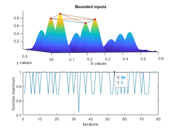
Plot of bounded inputs:

% Study 3 -Increasing Ga iterations

options =optimoptions('ga');
options=optimoptions(options,'populationsize',200);

tic
for i =1:Num_case
    [inputs,fopt(i)]=ga(@stalgmite,2,[],[],[],[],[0;0],[0.6;0.6],[],[],options);
    xopt(i)=inputs(1);
    yopt(i)=inputs(2);
end

study3_time=toc;

figure(3)
subplot(2,1,1)
hold on
surfc(xx,yy,-f)
shading interp
xlabel('x Values')
ylabel('Y values')
plot3(xopt,yopt,-fopt,'Marker','o','markersize',5,'MarkerFaceColor','r')
title('optimum solution')

subplot(2,1,2)
plot(-fopt)
xlabel('iteration')
ylabel('function maximum')

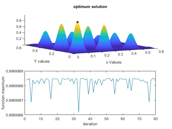
Plot of Optimum solution:

Conclusion :

With the help of matlab we can optimize the stalagmite function and find the global maxima of the function using GA

Project Link: https://skill-lync.com/myprojects/edit/119322