Week 4.1 - Solving second order ODEs

clear 
close
clc

b=0.05;
g=9.81;
l=1;
m=1;

% Initial comdition

theta_0=[0;5];

% time point
t_span = linspace(0,20,250);

% solve ODE
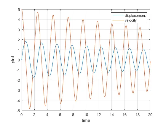
[t,results]=ode45(@(t,theta) ode_func(t,theta,b,g,l,m),t_span,theta_0);

figure(1)
plot(t,results(:,1))
hold on
plot(t,results(:,2))
ylabel('plot')
xlabel('time')
legend('displacement','velocity')
hold off
grid on

ct = 1;
for i = 1: length(results)
    THETA =  results(i,1);
    x0=0;
    y0=0;
x1=sin(THETA);
y1=-cos(THETA);

figure(2)
% Create the image that represent the position of the pendulum
plot(x1,y1,'o','markersize',20,'MarkerFaceColor','r') %Marker cammand used to create sphere
hold on
plot([x0 x1],[y0 y1],'linewidth',3)
plot([-.5 .5],[0 0],'linewidth',5)
axis ([-1.5 1.5 -2 1])
pause(0.10)
hold off
M(ct)=getframe;
ct=ct+1;
    
end

movie(M)
videofile=VideoWriter('simplependulum.avi','Uncompressed AVI');
open(videofile)
writeVideo(videofile,M)
close(videofile)


https://youtu.be/SajSUw2Q304

Youtube link:

https://youtu.be/SajSUw2Q304