Week 5 - Genetic Algorithm

what is GA in Matlab

In MATLAB, the ga function is used to perform genetic algorithm (GA) optimization, which is a heuristic(by trial and error) search and optimization technique inspired by natural evolution principles like selection, crossover, and mutation.

[x, fval] = ga(fitnessFunction, nvars)

[x, fval] = ga(fitnessFunction, nvars, A, b, Aeq, beq, lb, ub, nonlcon, options)

Parameters:

1. Fitness function:

A handle to the objective (fitness) function to minimize. It is defined as:

f = fitnessFunction(x)

where x is the input variable(vector) and f is the scalar output value which we need to minimize.

2. nvars:

number of variables to minimize.

3.A,B(optional):

Linear inequality constraints in the form $A \cdot x \leq b$A⋅x≤B.

when dealing with optimization problems the maxima or minia is written with inequalities as we learned i numerical methods and optimization.

4.Aeq, beq:

Linear equality constraints in the form $\mathrm{Aeq.x=Beq.}\mathrm{<br>}\mathrm{<br>}\mathrm{<br>}\mathrm{<br>}\mathrm{<br>}\mathrm{<br>}\mathrm{<br>}\mathrm{<br>}\mathrm{<br>}$

5.ub,lb:

the upper and lower bounds to the optimization.

6:nonlcon:

if any non linear constraints exists then provide these as nonlcon[non linear constraints];

7. Options:

Optimization options, specified as the output of optimoptions or a structure.

in our perticular case we used option to control the population size to 300.

In simple terms, the ga function in MATLAB works like nature's way of solving problems, inspired by how species evolve over time. Here's how it works, step by step:

1. Start with a Random Population

Imagine you're trying to find the best solution to a problem, but you don't know where to start. So, MATLAB creates a group of random "candidates" (called a population) that might be possible solutions. Think of these candidates as "wild guesses."

2. Evaluate Fitness

Each candidate solution is tested to see how "good" it is for solving the problem. This is done using a fitness function you provide.
For example:

• If you're minimizing cost, lower cost means higher fitness.
• If you're maximizing something (like profit), higher profit means better fitness.

3. Select the Best Candidates

Just like in nature, where the strongest individuals are more likely to survive and reproduce, MATLAB selects the "best" candidate solutions (the ones with higher fitness scores) for the next step.

4. Combine and Mutate

Now, the selected candidates "reproduce" to create new solutions. This happens in two ways:

• Crossover: Two solutions combine their "genes" (parts of their values) to create a new solution.
  Example: If one solution is 5 and another is 10, the child might be 7 (a mix of the two).
• Mutation: Random changes are made to some solutions to introduce variety.
  Example: If a solution is 7, it might randomly change to 8.

These steps ensure that new solutions are created that might be better than the old ones.

5. Replace Old Population

The new solutions replace the old population, and the process repeats. Over time, the solutions evolve, getting better and closer to the optimal answer.

6. Stop When It's "Good Enough"

The process keeps going for a certain number of "generations" or until the solutions stop improving significantly. At this point, MATLAB picks the best solution from the population and says, "This is the best answer I found!"

Example in Real Life

Imagine you're trying to guess the combination for a locked safe, but you don’t know the exact numbers. Here's what happens:

• You start with random guesses.
• You evaluate how close each guess is to opening the lock.
• You keep the better guesses and combine or tweak them to make new guesses.
• Over time, your guesses get closer and closer to the correct combination.

Why Use GA?

Genetic algorithms are helpful when:

• The problem is too complex to solve with standard math.
• There are lots of possible solutions, and you don't know where to start.
• The solution space is messy, with ups and downs (like hills and valleys).

The ga function mimics evolution to zero

Mutation in MATLAB's GA Toolbox

The MATLAB GA toolbox provides built-in mutation operators. The mutation is controlled by:

• Mutation function: Specifies how mutation should be applied.
• Mutation rate: Determines the likelihood of mutation occurring for a gene.

Steps in Built-in Mutation:

1. Selection of genes: A probability (mutation rate) determines which genes in the population will undergo mutation.
2. Mutation application: The mutation function modifies the selected genes. Examples of mutation functions include:
• Gaussian Mutation: Adds a random value drawn from a Gaussian distribution.
• Uniform Mutation: Replaces a gene with a random value within its bounds.

Common options include:

• PopulationSize: Number of individuals in each generation.
• MaxGenerations: Maximum number of iterations.
• EliteCount: Number of best individuals preserved between generations.
• CrossoverFraction: Fraction of population for crossover.
• MutationFcn: Custom mutation function.

Optimizing ga:
we finetuned the ga algorithm by using an options object;
for example
Common options include:
PopulationSize: Number of individuals in each generation.
MaxGenerations: Maximum number of iterations.
EliteCount: Number of best individuals preserved between generations.
CrossoverFraction: Fraction of population for crossover.
MutationFcn: Custom mutation function.
Function Called:
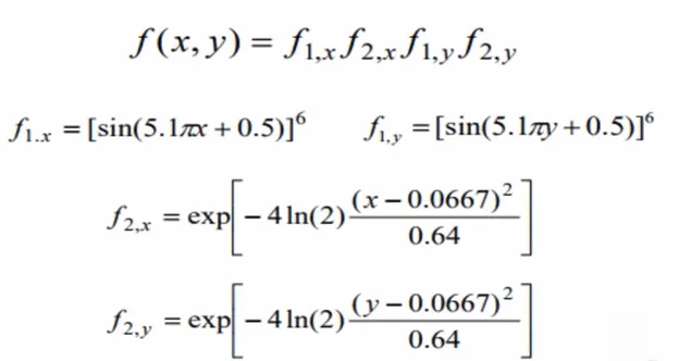
Stalagmite function
function f = stalagmite(input)
x = input(1);
y = input(2);
term1 = (sin(5.1*pi*x + 0.5)).^6;
term2 = (sin(5.1*pi*y + 0.5)).^6;
term3 =  exp(-4*log(2)*(x-0.0667).^2 / (0.64));
term4 = exp(-4*log(2)*(y-0.0667).^2 / (0.64));
f = -(term1 * term2 * term3 * term4);
end 
% it is important to note that the ga function optimizes the problem space and returns a minima of the 
function. Here the problem is to find the maxima, for this we just put a minus to get the maxima of the
function.
Here we set the x and y value to be determined in the main code, where in the main code we created an vector space from 0 to 0.7 of 150 iterations.
these are our randon sample space for both x and y.

The main code is pretty straight forward

for the first iteration:

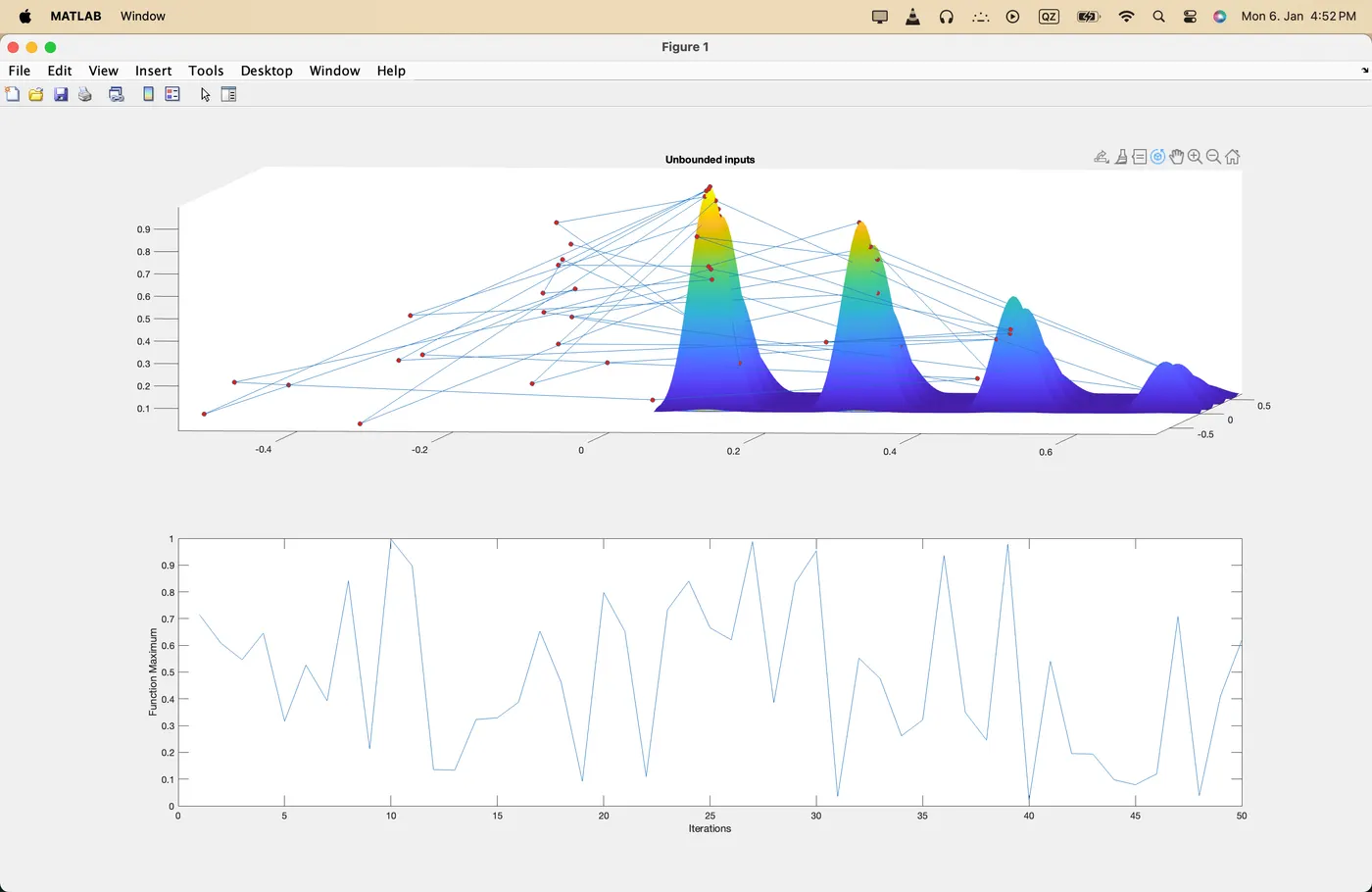
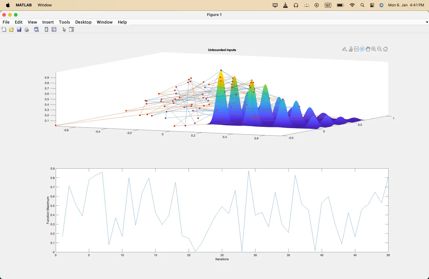
we create a sample space of random variables from 1 to 0.7 consisting of 150 numbers;set the iterations to 50 and call the ga with fitness function

uses the stalagmite function which we created using inputs x,y

for the second iteration:

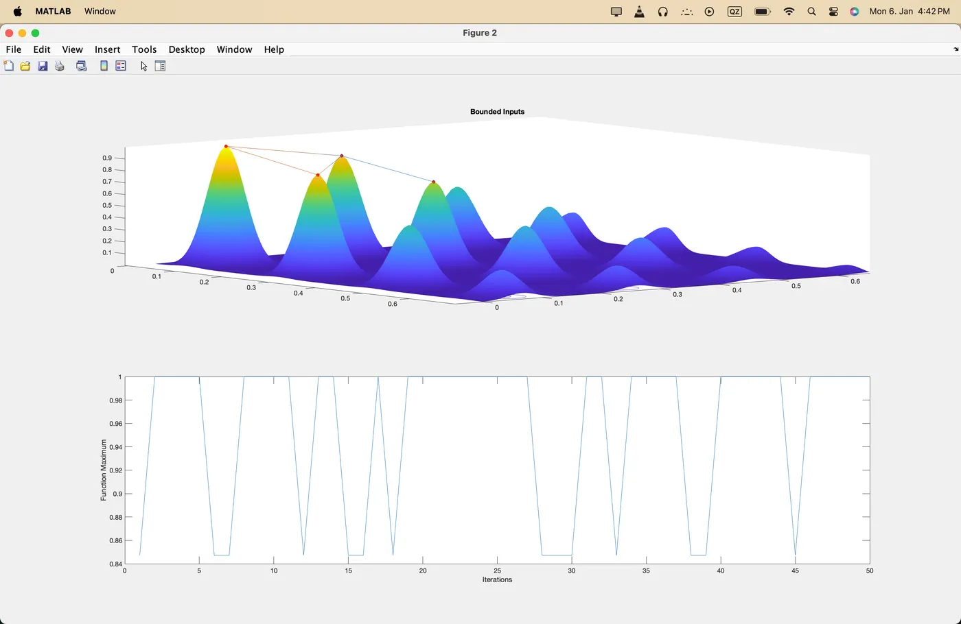
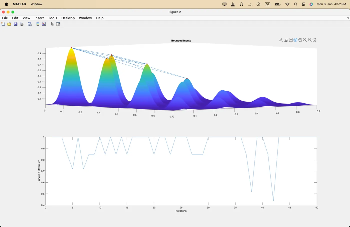
for the second itertion we just give lower bounds as 0 and upper bounds as 0.7;

for the 3rd iteration:

for the 3rd one we set the population size as 300 in the ga input argument.

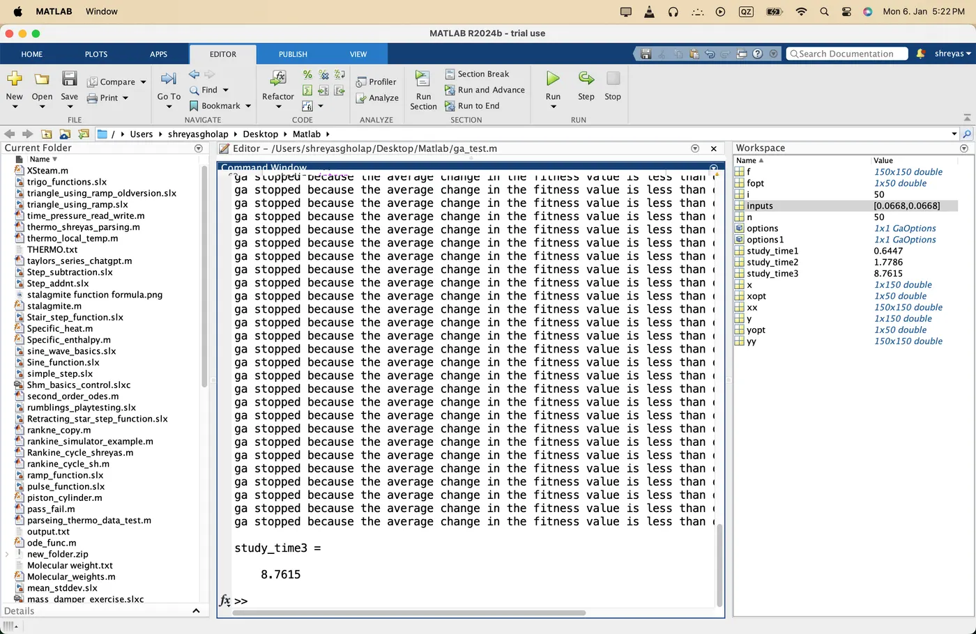
for runtime we use tic and toc where tic is used to start the clock before ga loop and toc is used to stop

it for every iteration.

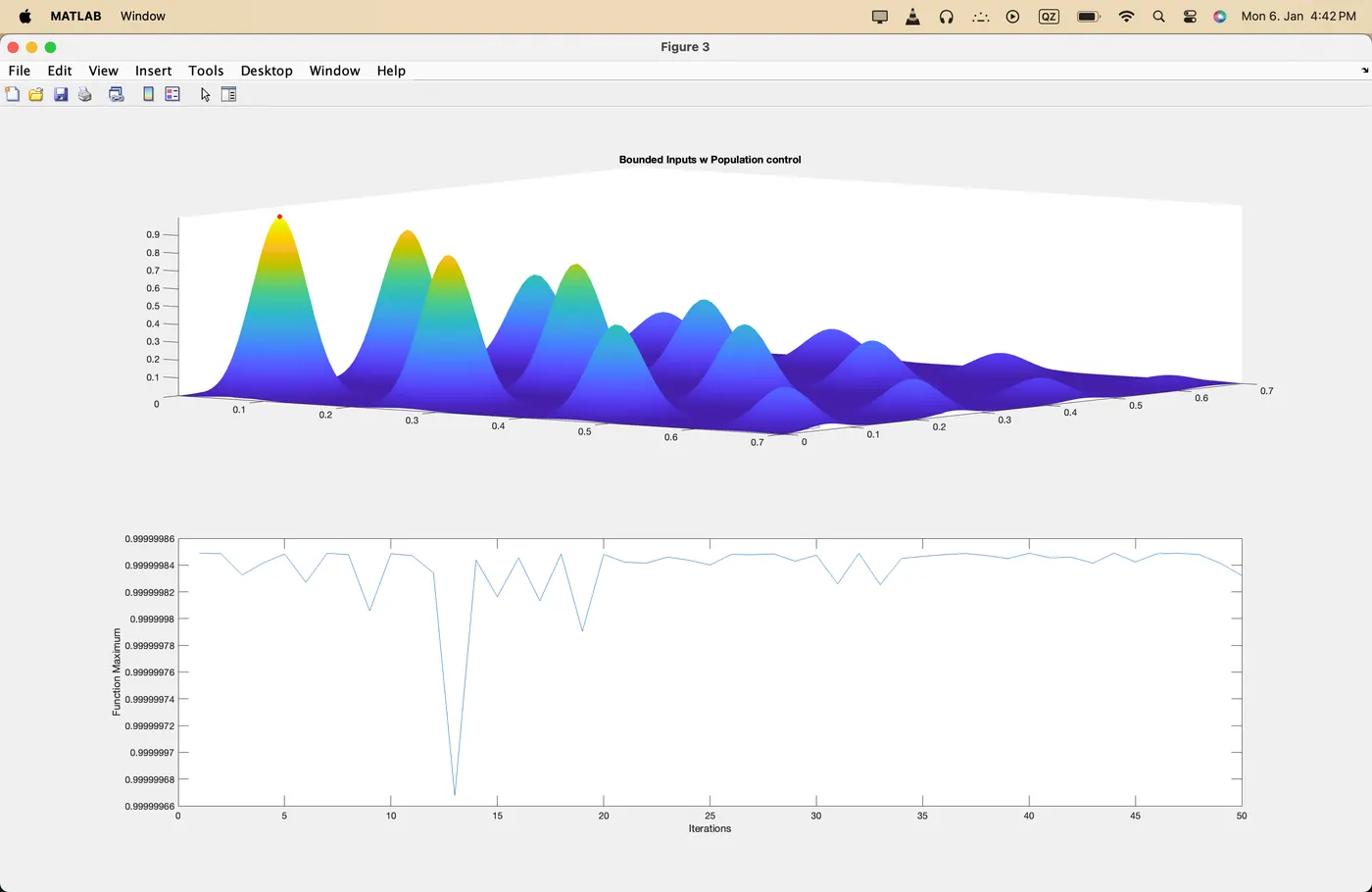
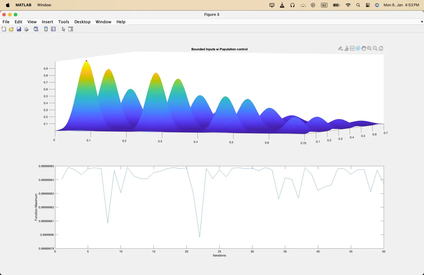
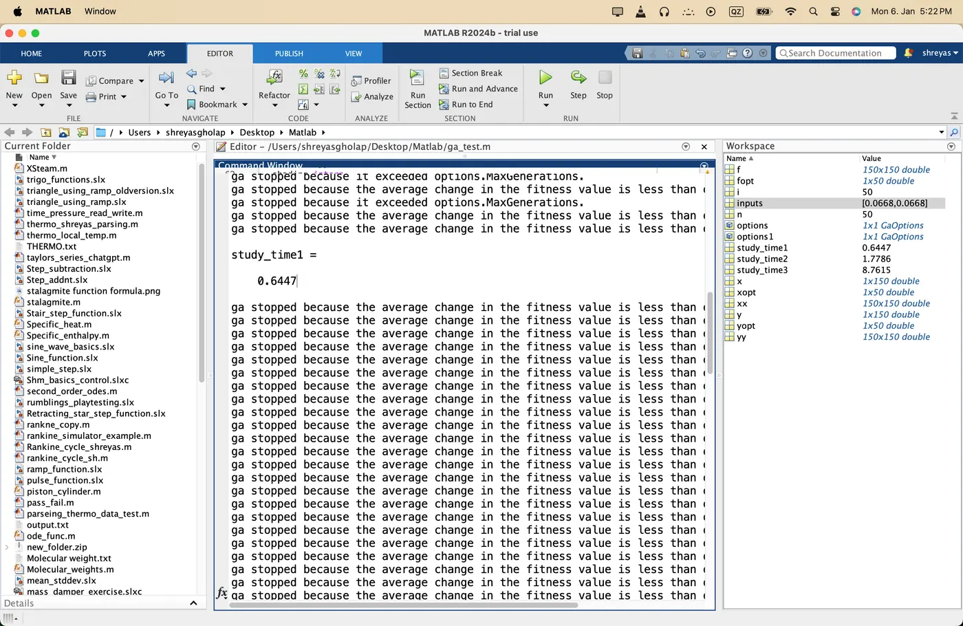
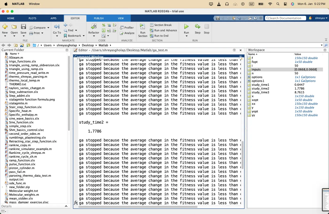
Main code:

clear all
close all
clc
%Study1: Without constraints and population control.
%Defining search space 
x = linspace(0,0.7,150);
y = linspace(0,0.7,150);
n = 50;  %Number of Iterations to be run 
f = get_stalagmite(x,y);
%creating 2D Mesh
[xx,yy] = meshgrid(x,y);
tic
%Evaluating the stalagmite function s
for i =1:n;
[inputs, fopt(i)] = ga(@stalagmite,2);%here 2 denotes no of inputs which are x,y
xopt(i) = inputs(1);
yopt(i) = inputs(2);                                                                                                                   
   
end 
study_time1 = toc
figure (1)%we plot the graph taking xopt and yopt as axis
subplot (2,1,1)
hold on % Hold the graph
surfc(xx,yy,f)
shading interp %inter argument removes the gridlines on meshcurve leading to better visualization of graph
title ('Unbounded inputs')
plot3(xopt, yopt, abs(fopt),'marker', 'o', 'markersize', 5, 'markerfacecolor','r')
subplot(2,1,2)
plot (abs(fopt))
xlabel('Iterations')
ylabel('Function Maximum')


%Study2:With Upper and Lower bounds:
%Defining search space 
x = linspace(0,0.7,150);
y = linspace(0,0.7,150);
n = 50; %Number of Iterations to be run 
f = get_stalagmite(x,y);
%creating 2D Mesh
[xx,yy] = meshgrid(x,y);
tic
%Evaluating the stalagmite function 
for i =1:n;
[inputs, fopt(i)] = ga(@stalagmite, 2, [], [],[],[], [0;0],[0.7;0.7]);
xopt(i) = inputs(1);
yopt(i) = inputs(2);                                                                                                                   
   
end 
study_time2 = toc
figure (2)
subplot (2,1,1)
hold on
surfc(xx,yy,f)
shading interp
title ('Bounded Inputs')
plot3(xopt, yopt, abs(fopt),'marker', 'o', 'markersize', 5, 'markerfacecolor','r')
subplot(2,1,2)
plot (abs(fopt))
xlabel('Iterations')
ylabel('Function Maximum')



%Study3: With upper and lower bounds and population size control
options = optimoptions ('ga');
options1 = optimoptions (options, 'PopulationSize', 300);
tic
%Evaluating the stalagmite function 
for i =1:n; %n =Number of Iterations to be run 
[inputs, fopt(i)] = ga(@stalagmite,2,[],[],[],[], [0;0],[0.7;0.7], [], [], options1);
xopt(i) = inputs(1);
yopt(i) = inputs(2);                                                                                                                   
   
end 
study_time3 = toc
figure (3)
subplot (2,1,1)
hold on
surfc(xx,yy,f)
shading interp
title ('Bounded Inputs w Population control')
plot3(xopt, yopt, abs(fopt),'marker', 'o', 'markersize', 5, 'markerfacecolor','r')
subplot(2,1,2)
plot (abs(fopt))
xlabel('Iterations')
ylabel('Function Maximum')
%end 

Case1: with unbounded inputs:
iteration 1
here it can be noted that the ga function being unoptimized results are all over the sample space
the format used for this ga is [inputs fopt]=ga(function,nvars)
figure 2 with bounded inputs
iteration 1
the format of ga used in this is [inputs fopt]=ga(fun,nvars,A.b.Aeq.beq lb,ub))
here we used the default pop size which is 50 for both x and y inputs. As our study size was small our output is local maxima and not global maxima. Hence we did a study 3 with increased pop size which helped us arrive at better results withi the sample size.Now for plotting the graphs, "figure command is used for a new figure window, “subplot" is used for dividing the window in parts, and here it divides the figure window In two parts. In the first half two graphs are plotted in a single graph using the "hold” on command, "surfc” command is used which plots a surface graph and the other graph is 3 dimensional line plat for this the command used is "plot3 X and Y label is given along with the title. Now in the second half a 1D plot is generated of values stored in “fopt” using the “plot” command and then label the x-axis and y-axis.
iteration 2
Figure 3 with bounded inputs and population controls:
iteration 2:

Runtime:
the runtime which we calculated with tic and toc command gave the following results:
As we can see from our output the study time increases with number of iterations. 
We understood how to optimize our statistical model using random samplng in ga.