Week 4.1 - Solving second order ODEs
Youtube link: https://www.youtube.com/watch?v=b8VB5x_4FhU&ab_channel=shreyasgholap
Main Code
%inputs
L=1; %length of pendulum arm
g=9.81; %Acceleration due to gravity
m=0.1; %mass attached to arm of pendulum(or mass at end of spring)
b=0.05; %Damping coeff
%initial conditions
theta_0=[0;3]; %semicolon represents columnso 0 and 5 are 2 columns representing initial displacement and initial velocity
%initial displacement is 0 and initial velocity is 5m/s
t_span=linspace(0,20,500);
% we create a vector of time from 0 to 20 seconds having 500 iterations
%these 0 to 20 are our boundry conditions for solving the ode
%ode solver
[t,results]=ode45(@(t,theta) ode_func(t,theta,b,g,L,m),t_span,theta_0);
%We call built in ode solver function ode45 with input arguments
%1. t,theta: are the main variables in our ode. main inputs.
%2. ode_func: we call a created function where we just used substitution to
%convert the 2nd order ode into 1st order odes.
%3.t_span and theta_0 are just the final and initial conditions for solving ur ode
%4 we need to keep in mind that the initial condition theta_0 column matrix corresponds to
%column matrix in the ode function definition else we would get wrong results.
figure(1)
plot(t,results(:,1),"Color",'r');
hold on
%plot the displacement. here the results array contains 2 column 1st is
%the displacement which we call using the (:,1)denoting all rows from 1st
%column vs time
plot(t,results(:,2),"Color",'b');
%plotting the velocity called from the second column of the ressults array
%vs time called from the second column of the results array vs time
ylabel('Results')
xlabel('time')
legend("Angular displacement","Angular velocity")
%we use legend to make plot easy to understand giving names to x and y
%axis
% For creating animation and saving it to video file:
%set counter variable starting from 1
ct = 1;
% we take our results from the inital plot representing displacement
% and create a for loop for all the vaues we got for its displacement.
for i = 1:length(results(:,1))
%we set the initial values as 0 so our pendulum starts from
x0 = 0;
y0 = 0;
%one end of the arm is fixed at 0
%the other end oscillates to following equation
x1 = L*sin(results(i,1));
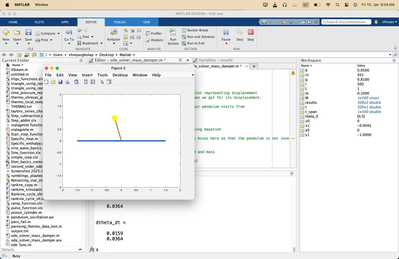
y1 = -L*cos(results(i,1)); %we use minus here so that the pendulum is not inverted(see pics in mistakes)
% Plotting the animation background,mass and arm of pendulum
figure(2)
plot([-1.5 1.5],[0 0],'linewidth',5)
hold on
plot([x0 x1],[y0 y1],'linewidth',3)
hold on
plot(x1,y1,'o','markersize',20,'markerfacecolor','y') %for plotting the
%mass on
%pendulum
axis([-2 2 -2 2])%we set axis so we can see the graph
pause(0.003) %we use pause so that the graph stop at the specified time(0.03sec)
%we do this so we get an animation of subsequent graphs
hold off
M(ct) = getframe(gcf);
ct = ct+1;
end
% Converting the animation into a movie
movie(M)%gathers all frames
videofile = VideoWriter('pendulum_oscillation.avi','Uncompressed AVI');%creates a file in specified format and saves it
open(videofile)%opens said file
writeVideo(videofile,M)%writes data in the file
close(videofile)%closes it
Ode_function:
function [dtheta_dt] = ode_func(t,theta,b,g,L,m)
theta1=theta(1)
theta2=theta(2)
dtheta1_dt=theta2
dtheta2_dt=-(b/m)*theta2-(g/L)*sin(theta1)
dtheta_dt=[dtheta1_dt;dtheta2_dt] %important to note dtheta1_dt corresponds to
%displacement and dtheta2_dt to
%velocity,seperated into 2 columns using;
%operator
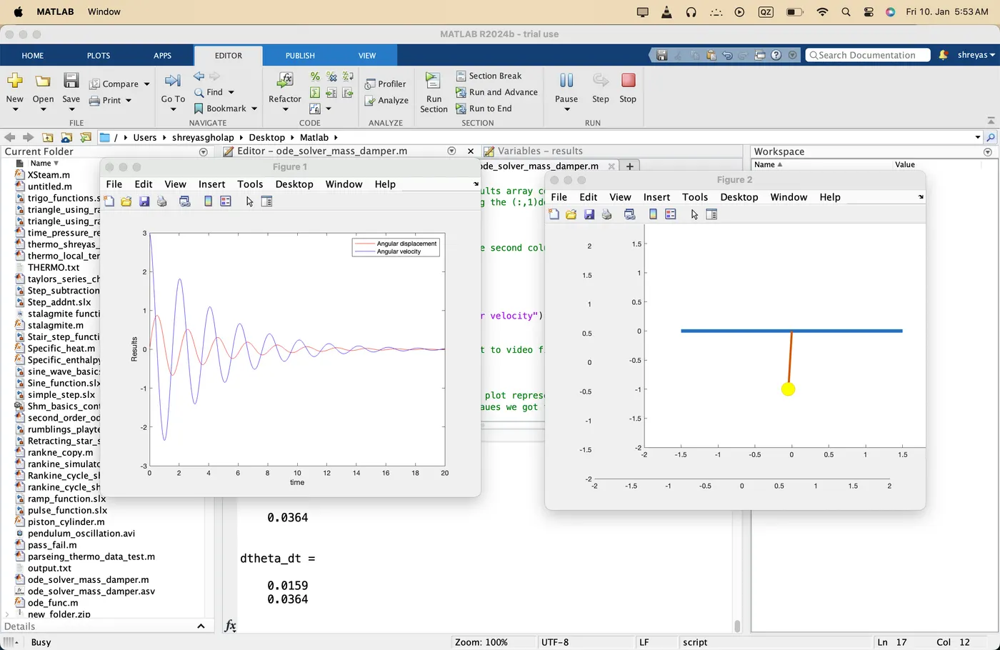
plot and animation
Mistakes made:
used smaller damping coefficient and wrong initial velocity also time taken was 10 secs instead of 20 as given in problem
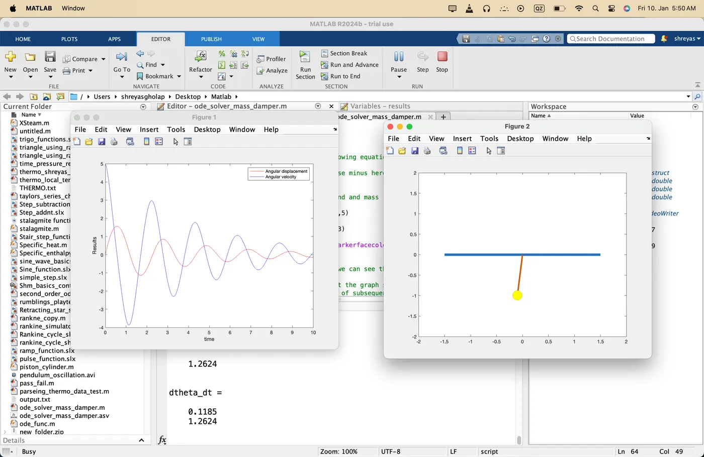
Did not use minus sign(see code for detailed explaination)