Week 5 - Genetic Algorithm

AIM:- Try to understand the concept of genetic algorithm by referring to varius sources before you attend this challenge. Look out for information regarding stalagmite function and ways to optimise it.

DESCIRPTION:-

The genetic algorithm is inspired by the process that drives biological evolution. The process of evolution starts with the selection of fittest individuals from a population. Then they produce offspring which inherit the characteristics of the parents and will be added to the next generation. If parents have better fitness, their offspring will be better than parents and have a better chance at surviving. This process keeps on iterating and at the end, a generation with the fittest individuals will be found. And this is the main working principle for the algorithm because at each step, the genetic algorithm selects randomly from the current population to be parents and uses them to produce the children for the next generation. Over successive generations, the population evolves toward an optimal solution. The genetic algorithm can be applied to solve a variety of optimization problems that are not well suited for standard optimization algorithms, including problems in which the objective function is discontinuous, nondifferentiable, stochastic, or highly nonlinear.

The genetic algorithm uses three main types of rules at each step to create the next generation from the current population:

• Selection rules select the individuals, called parents, that contribute to the population at the next generation.
• Crossover rules combine two parents to form children for the next generation.
• Mutation rules apply random changes to individual parents to form children.

Codes:-

main function:-
function y= func1(x)
    f1=(sin((5.1*pi*x(:,1)+0.5))).^6;
    f2=(sin((5.1*pi*x(:,2)+0.5))).^6;
    f3=exp(-4*log(2)*((x(:,1)-0.0667).^2)/0.64);
    f4=exp(-4*log(2)*((x(:,2)-0.0667).^2)/0.64);
    y=-f1.*f2.*f3.*f4;
end

MAIN CODE:-
 x=linspace(0,0.6,100);              %x range
y=linspace(0,0.6,100);              %y range
[xx,yy]=meshgrid(x,y);              %creating a meshgrid with x and y values
f=zeros(100);                       %preinitialising f matrix to make the code faster
for i=1:length(xx)
    for j=1:length(yy)
        c(1)=xx(i,j);
        c(2)=yy(i,j);
        f(i,j)=func1(c);           %calling func1 function to return its value
    end
end
 
options=optimoptions('ga');
%changing population size from default 50 to 200
options=optimoptions(options,'Populationsize',200);
%changing function creation function to use <= equalities, more about this
%at the end of the code
%options=optimoptions(options,'CreationFcn', @gacreationlinearfeasible);
%changing function tolernce value to terminate optimization
options = optimoptions(options,'FunctionTolerance',1e-4);
 
iter=25;                        %number of iterations
coor=zeros(iter,2);             %preinitialising coordinate matrix to make the code faster
fmax=zeros(iter,1);             %preinitialising fmax matrix to make the code faster
for i=1:iter
    %calling ga function with linear inequalities. more about this at the
    %at the end of the code
    %[coor(i,:),fmax(i)]=ga(@func1,2,[1,-1],0,[],[],[0;0],[0.6;0.6],[],[],options);
    %calling ga function with just lower and upper bounds
    [coor(i,:),fmax(i)]=ga(@func1,2,[],[],[],[],[0;0],[0.6;0.6],[],[],options);
end
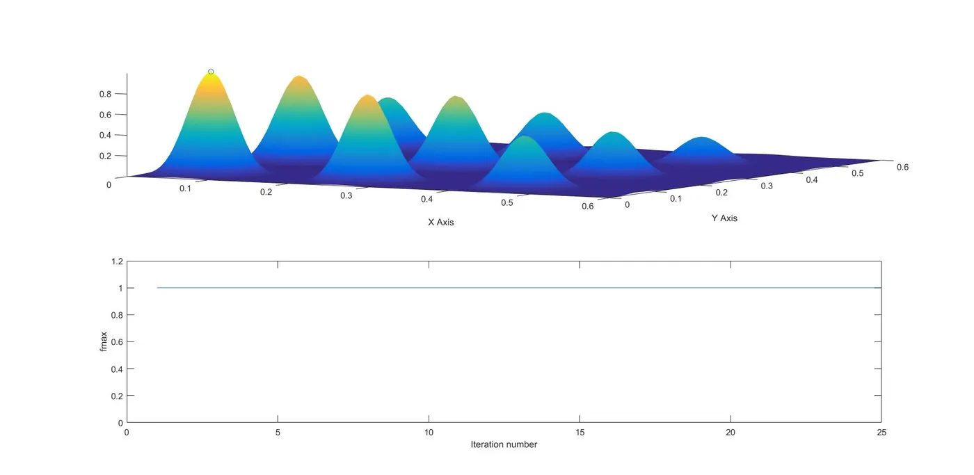
subplot(2,1,1)                  %1st plot
hold on
surfc(xx,yy,-f)                 %plotting the contours of func1
shading interp
plot3(coor(:,1),coor(:,2),-fmax,'o')
xlabel('X Axis');
ylabel('Y Axis');
subplot(2,1,2)                  %2nd plot
plot(-fmax)
axis([0 iter 0 1.2])
xlabel('Iteration number');
ylabel('fmax');

Conclusion:-

In the main code , The stalagmite function is classified into 3 sectors,

they are

1-unbounded inputs.

2-bounded inputs.

3-bounded inputs with increased population

In the unbounded inputs ,they dont have any limits ,the values are distributed outside the limits.

In the bounded inputs, they have limits, so the values are distributed inside the limits.

In the bounded inputs with increased population, the number of iteration are increased .