Week 2- 2R Robotic Arm Challenge
Aim
To write a program in Matlab to simulate the forward kinematics of a 2R Robotic Arm.
Theory
Robotic Arm
A robotic arm is a type of mechanical arm, usually programmable, with similar functions to a human arm; the arm may be the sum total of the mechanism or may be part of a more complex robot. The links of such a manipulator are connected by joints allowing either rotational motion or translational displacement. The links of the manipulator can be considered to form a kinematic chain. The terminus of the kinematic chain of the manipulator is called the end effector and it is analogous to the human hand.
Kinematics of Robot
Robot kinematics applies geometry to the study of the movement of multi-degree of freedom kinematic chains that form the structure of robotic systems. The emphasis on geometry means that the links of the robot are modeled as rigid bodies and its joints are assumed to provide pure rotation or translation.
Robot kinematics studies the relationship between the dimensions and connectivity of kinematic chains and the position, velocity and acceleration of each of the links in the robotic system, in order to plan and control movement and to compute actuator forces and torques. The relationship between mass and inertia properties, motion, and the associated forces and torques is studied as part of robot dynamics.
Types of Kinematic
There are two type of kinematics,they are
⦁ Forward kinematics
⦁ Inverse kinematics
Forward Kinematics
Forward kinematics specifies the joint parameters and computes the configuration of the chain. For serial manipulators this is achieved by direct substitution of the joint parameters into the forward kinematics equations for the serial chain. For parallel manipulators substitution of the joint parameters into the kinematics equations requires solution of the a set of polynomial constraints to determine the set of possible end-effector locations.
Inverse kinematics
Inverse kinematics specifies the end-effector location and computes the associated joint angles. For serial manipulators this requires solution of a set of polynomials obtained from the kinematics equations and yields multiple configurations for the chain. The case of a general 6R serial manipulator (a serial chain with six revolute joints) yields sixteen different inverse kinematics solutions, which are solutions of a sixteenth degree polynomial. For parallel manipulators, the specification of the end-effector location simplifies the kinematics equations, which yields formulas for the joint parameters.
Velocity kinematics
From the reference, to Jacobian Matrix theory,The robot Jacobian results in a set of linear equations that relate the joint rates to the six-vector formed from the angular and linear velocity of the end-effector, known as a twist. Specifying the joint rates yields the end-effector twist directly.
The inverse velocity problem seeks the joint rates that provide a specified end-effector twist. This is solved by inverting the Jacobian matrix. It can happen that the robot is in a configuration where the Jacobian does not have an inverse. These are termed singular configurations of the robot.
Workspace of Robot.
The workspace of robot manipulator is defined as the set of points that can be reached by its end‐effector. Put in other words, the workspace of a robot is the space in which the mechanism is working.
Linkage
A mechanical linkage is an assembly of bodies connected to manage forces and movement. The movement of a body, or link, is studied using geometry so the link is considered to be rigid.[1] The connections between links are modeled as providing ideal movement, pure rotation or sliding for example, and are called joints. A linkage modeled as a network of rigid links and ideal joints is called a kinematic chain.
Linkages may be constructed from open chains, closed chains, or a combination of open and closed chains. Each link in a chain is connected by a joint to one or more other links. Thus, a kinematic chain can be modeled as a graph in which the links are paths and the joints are vertices, which is called a linkage graph.
Basically Mechanical linkages are usually designed to transform a given input force and movement into a desired output force and movement.
Angle Between the Linkage
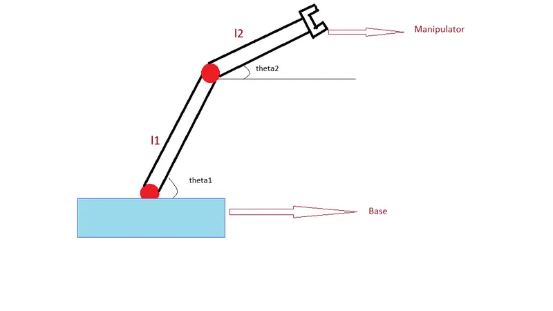
we have assumed that the first angle with which is supported in ground and there may or may not be a linkage but that has a certain degree that we take as and length we use as L1.
Above first link there is an another link which has manupulator have an angle ofand the length will be L2.as shown in Figure.
Program for two arm robotic manipulator
% forward kinematics of a 2 rotation arm manipulator
clear all
close all
clc

% inputs
l1=1;
l2=0.5;
theta1=45
theta2=30

% coordinates

x0=0;
y0=0;

x1=l1*cosd(theta1)
y1=l1*sind(theta1)

x2=x1+l2*cosd(theta2);
y2=y1+l2*sind(theta2)

% plotting
line([x0 x1],[y0 y1],'linewidth',3,'color','r');
line([x1 x2],[y1 y2],'linewidth',3,'color','b');
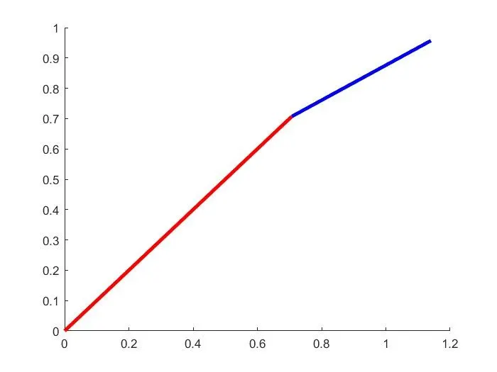
After executing the above program the followinng plot can be diagram was observed for two rotation robotic arm.
Figure shown the value for the input which used was fixed
L1 = 1
L2 = 0.5
Theta1 =45 degree
Theta2 =0 degree
Which the values are fixed in this case.
Progarm for forward kinematics with for loop.
close all
clear all
clc

% craeting animation  of forward kinematics.
% animations -- its objescctive to have multipule values of theta1 and
%____theta2 for an 2r robotic arm

%inputs
l1=1
l2=0.5
theta1=linspace(0,90,4);
theta2=linspace(0,90,4);
ct=1;
for i=1:length(theta1);
    THETA1=theta1(i);
    for j=1:length(theta2);
    THETA2=theta2(j);

    x0=0
    y0=0

    x1=l1*cosd(THETA1);
    y1=l1*sind(THETA1);

    x2=x1+l2*cosd(THETA2);
    y2=y1+l2*sind(THETA2);

    % plotting.

   %line([x0 x1],[y0 y1],'linewidth',3,'color','b');
   %line([x1 x2],[y1 y2],'linewidth',3,'color','r');

  % figure(ct)
  % add command 'hold on' 'plot command'
  % line([x0 x1],[y0 y1],'linewidth',3,'color','b');
  % line([x1 x2],[y1 y2],'linewidth',3,'color','r');
  % ct=ct+1


 plot([x0 x1],[y0 y1],[x1 x2],[y1 y2],'linewidth',3);
 axis([-0.1 1.5 0 1.5]);
 pause(0.03)
 m(ct)=getframe(gcf)
  ct=ct+1


    end

end

movie(M)
videofile = VideoWriter('Forward kinematics 2r robotics.avi','uncompressed AVI');

open(videofile)
writeVideo(videofile,M)
close(videofile)
Detailing the Program
Input
First things need to consider is input which we have assumed and the boundries,
In program I have given the input values are
L1 = 1
L2 = 0.5
Theta1 = linspace(0,90,10);
Theta1 =THETA1= degree varies from 0 to 90 equally serepated 10 values
Theta2 = linspace(0,90,10);
Theta2 =THETA2 = degree varies from 0 to 90 equally serepated 10 values
For Loop
We have using For loop for to defain a certain repeated work to the matlab with cetain restrictions.
Plotting
Plotting is like we are ploting the graph with respect to the result which we have been generated. Basically Create a simple line plot and label the axes. Customize the appearance of plotted lines by changing the line color, and the line style.
Making an Animation
Firstly we need to get frame from the program so before starting loop we need to get frame so that we have use this command,
M(ct) = getframe(gcf);After that only we will be using loop command,
ct = ct+1;From collection of that frame the animation will be created with certain lag or pause in that frame using Command before the get frame Command,
pause(0.03)
so the frame will have a pause for defined seconds.
Errors Faced While Programming
I haver faced errors during writing program for movie making and in that had difficulty to store the video.
Also confused to understand the for loop command while executing it.
Video Link
Conclusion
I have concluded that by using matlab commands can simulate the Forward kinematics for 2R Robotic Arm