Week 5 - Genetic Algorithm

Aim-write code for global maxima of stalagmite function and also explain what is genetic algoritham.

Objective-

1. write a code to optimize stalagmite function and also find global maxima
2. what is genetic algorithm and 'ga syntax ' used in metlab
3. plot the graph for global maxima and three studies

Theory-

Optimization -To get maximum possibal output optimization are used

aplication of optimization -mechanics, economics finance,machine learing,artificial intelligence,control engineering

Genetic Algoritham - Genetic algoritham is metode for solving both constraind and unconstrained optimization problems based on the natural selection process that mimics biological evolution you can apply the genetic algorithem to solve problem that are not well suited for standard optimization algoritham including problem in which objective function discontinuos, nondifferentiable and highly nonlinear.

The genetic algoritham works on the natural sselection where the fittest individual are selected for reproduction in order to produce offspring of next generation.

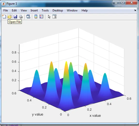
Stalagmite Function -

% stalagmite function
function [f]=stalagmite(input_vector)
x = input_vector(1);
y = input_vector(2);

b1=(sin((5.1*pi*x)+0.5))^6;
b2=(sin((5.1*pi*y)+0.5))^6;
b3=exp(-4*log(2)*((x-0.0667)^2)/0.64);
b4=exp(-4*log(2)*((y-0.0667)^2)/0.64);

f=-(b1*b2*b3*b4);
end

Codes for global maxima-

clear all
close all
clc
%  creating  1D array
x=linspace(0,0.6,150);
y=linspace(0,0.6,150);


% from above 1D arry creat 2D arry
[xx,yy]=meshgrid(x,y);

% number of cases
 n=50;
% evaluating stalagmite function
for     i =1:length(xx)
   for  j=1:length(yy)
        input_vector(1)=xx(i,j);
        input_vector(2)=yy(i,j);
        f(i,j) = stalagmite(input_vector);
        
   end
end


% study 1
tic
for  i=1:n
    [inputs,fopt(i)]=ga(@stalagmite,2);
    xopt(i) =inputs(1);
    yopt(i) =inputs(2);
end
study1_time =toc;
figure(1)
subplot(2,1,1)
hold on
surfc(xx,yy,-f)
shading interp
xlabel('X-axis')
ylabel('Y-axis')
title('unbound inputs')
plot3(xopt,yopt,-fopt,'marker','o','MarkerSize',6,'MarkerFaceColor','r')
subplot(2,1,2)
plot(-fopt)
xlabel('no.of iterations')
ylabel('function maximum')

%study 2 upper and lower bounds
tic
 for i= 1:n
     [inputs,fopt(i)]=ga(@stalagmite,2,[],[],[],[],[0;0],[1;1]);
     xopt(i)= inputs(1);
     yopt(i)= inputs(2);
 end
 study2_time=toc;

 figure(2)
 subplot(2,1,1)
 hold on
 surfc(xx,yy,-f)
 shading interp
 xlabel('x-axis')
 ylabel('Y-axis')
 title('upper and lower bounds')
 plot3(xopt,yopt,-fopt,'marker','o','MarkerSize',6,'MarkerFaceColor','r')
 subplot(2,1,2)
 plot(-fopt)
 xlabel('no.of itertions')
 ylabel('function maximum')

 % study3 increasing iteration of ga
options = optimoptions('ga');
options = optimoptions(options,'PopulationSize',300);

tic
for i =1:n
    [inputs,fopt(i)]=ga(@stalagmite,2,[],[],[],[],[0;0],[1;1],[],[],options);
    xopt(i) = inputs(1);
    yopt(i) = inputs(2);
end
study3_time=toc;

figure(3)
subplot(2,1,1)
hold on
surfc(xx,yy,-f)
shading interp
xlabel('X-axis')
ylabel('Y-axis')
title('increasing iterations')
plot3(xopt,yopt,-fopt,'Marker','o','MarkerSize',5,'MarkerFaceColor','r')
subplot(2,1,2)
plot(-fopt)
xlabel('no.of iterations')
ylabel('function maximum')
hold off

code explanation-The code start from the basics cammands clear all, close all & clc

After that create 1D array x,y by using 'linspace' commmand

From the 1D array we create 2D array by using the 'meshgrid' command like xx & yy

After creating 2d array evaluate the stalagmite function and 'for loop' is used for the 'i' and again for loop is used for the initialize 'j'

input_vector value of xx,yy are define and this will form a stalagmite function and plot

Next step is get results for the 3 cases og genetic algoritm

To slove the loop for 50 iteration 'tic' and 'toc' commands are used

Then function created in the loop is plotted and different commands are used for the plot.like'surfc' command for xx,yy and function output and 'shading interp' command is used for hiding gridlines and obtain smooth and clean plot, subplot(21,,1)command is also used and this command used for the plot the multiple plot in same figure

plot3 commands plot the 3Dpoints at 'xopt,yopt and optimum value of function with 'o' shaped

above process follow for the case 2 with little changes

For the case-3 numbers of iteration are increased to 300 and syntax 'options=optimoptions('ga')

Results-

case1 – Statistical Behaviour

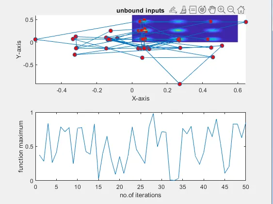
Red dots shows the values of co-ordinats of x,y varies each time iteration run

case 2- Statistical Behaviour with upper and lower bounds

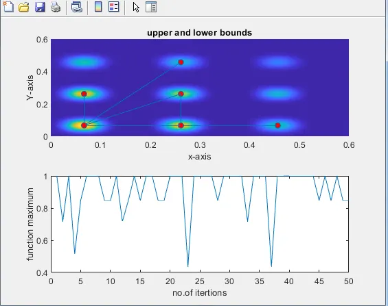
The red dots are less numbers as compare to privious plot,results providing upper and lower bound to function

case 3-Statistical Behaviour with increasing iterations of ga

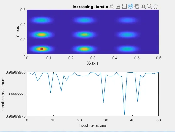
The numbers of iteration increasing to 300 and get global maxima of the function

and at that point x is 0.0668319 and y is 0.0668325 and z is 1

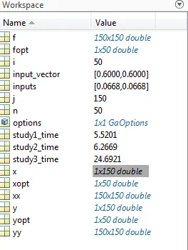
wokspace results-