Week 3 - Solving second order ODEs
Aim- To plot animation of simpal pendulum & plot the curve in betwen to velocity and angular displacement
Theory- for the animation we need 1st order equation but in the problem we have 2nd order equation.at first
this 2nd equation converts into the 1st order .
d^2θ/dt^2+(b/m)*dθ/dt+(g/l)*sinθ =0 .....(main equation )
b= damping coefficient
m=mass of bab
l= length of strings
g=gravity
after solving this equation
we got
dθ/dt=θ2
&
d^2θ/dt^2=-(b/m)*θ2-(g/l)*sinθ1
this two values and ode45 solver use for the creat animation of pendulum
Codes-
clear all
close all
clc

% inputs given values
   % mass of bob
   m=1;
   % length of string
   l=1;
   % damping coefficient
   b=0.05;
   % gravity
   g=9.81;
   % counter variable
   ct = 1;

% intial condition
theta_0=[0;3];

% time
t_span=linspace(0,20,500);

% ode function calling
[t,results] = ode45(@(t,theta)ode_func(t,theta,b,g,m,l),t_span,theta_0);

figure(1)
hold on
plot(t,results(:,1))
plot(t,results(:,2))
ylabel('y axis')
xlabel('x axis')
legend('displacement','velocity')
grid on
title('simpal harmonic motion')

theta2= results(:,1);
for i=1:length(theta2);
    theta_x=theta2(i);
    x0=0;
    y0=0;
    x1=l*sin(theta_x);
    y1=-l*cos(theta_x);

    %plot pendulum
    figure(2)
    plot([-0.5 0.5],[0 0 ],'color','r','linewidth',5);
    hold on
    plot([x0 x1],[y0 y1],'color','b','linewidth',3);
    hold on
    plot(x1,y1,'o','markers',20,'markerfacecolor','y')
    hold off
     axis([-1.5 1.5 -1.5 1.5]);
     pause(0.0003)
     grid on


    M(ct) = getframe(gcf);
    ct=ct+1;
end
   movie(M)
   videofile =VideoWriter('simple pendulum.avi','Uncompressed AVI');
   open(videofile)
   writeVideo(videofile,M)
   close(videofile)
code explanation -
- inputs the all given values like mass, length of string,gravity,damping coefficient etc
- then create yhe array of initial condition for velocity & displacement
- theta_0=[0;3] here in this 0 is displacement and 3 is velocity
- t_span=linspace(0,20,500)
- t-span command use to specifier as in the ode45 solver
- after the initial variables and inputs given solve the ode45 solver
- ode is nothing but ordinary differential equation
- ode45 is used to solve the ordinary function
- ode45 -syntex is
t_span is a time range
- [t,results] = ode45(@(t,theta)ode_func(t,theta,b,g,m,l),t_span,theta_0)
- after that plot figure
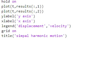
- after the plotting SHM ,create codes for animation of pendulun
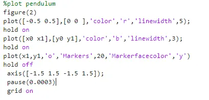
- after that create movie
movie(M)=plays the movies frames in array 'M' - video writer-this commands will create videofile of specific name
velocity vs displacement curve-
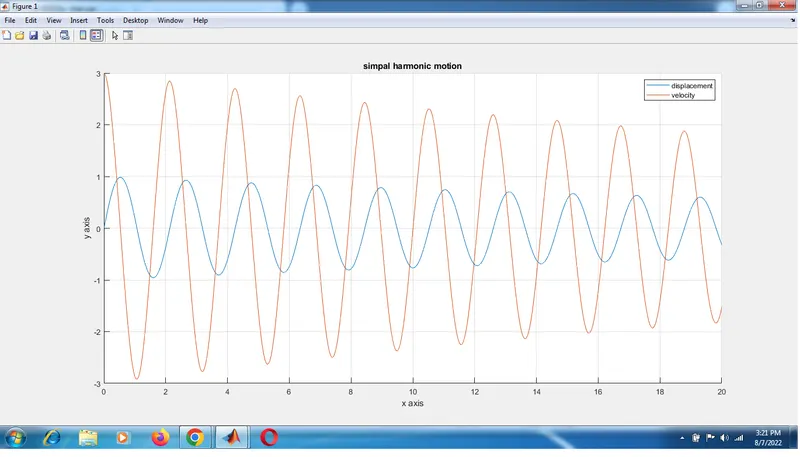
figuree shows that blue line show the displacement and its start from the zero
red line show the velocity bob and its start from point 3
conclusion- we got animation of pendulum by using the ode45 solver
https://drive.google.com/file/d/11iiSij4JkF_ORdeG-HwwkQjP5UiBAgvo/vie