Week 5 - Genetic Algorithm

CONCEPT OF GA:

Genetic algorithm is based on the theory of evolution. Like organisms produce offspring having traits from both the parents, they further have some mutations in the genes and adapt to the surroundings to survive, GA also uses these concepts to produce better solutions. The most fit individuals survive whereas the others perish.

GA also uses mainly the following operators to get results of an optimisation problem:

1. Selection

2. Mutation

3. Crossover

The advantage of GA as compared to calculus-based techniques is that GA works on a population of possible solutions. This makes it easier for GA to reach the global optimum value of an optimization problem. Moreover, GA can also be applied to problems which do not have an algebraic objective function.

SYNTAX IN MATLAB:

[x,fval,exitflag,output,population,scores] = gamultiobj(fitnessfcn,nvars,A,b,Aeq,beq,lb,ub,nonlcon,options)

x - output of the optimum points

fval - objective function values at the optimum points

exitflag - An integer value providing information about the stopping criteria triggered (i.e. max iterations reached, tolerance reached etc)

population - The population at the final iteration

scores - Score for the population at the final iteration

fitnessfcn- The objective function to optimize

nvars- No of independent variables in the fitnessfcn whose value has to be found

A,b - Matrices to specify the inequality constraints (if any) in the problem

Aeq,beq - Matrices to specify the equality constraints (if any) in the problem

lb - Lowest value which the independent variables are allowed to take

ub - Highest value which the independent variables are allowed to take

nonlcon - Non-linear constraints in the problem (if any)

options - Options to configure the operation of GA like Cross Over Ratio, Fitness function to be used, cross-over function to be used etc.

CODE:

clear all
close all
clc

%Defining search space
x = linspace(0,0.6,150);
y = linspace(0,0.6,150);
num_cases = 100;

%Creating a 2D mesh
[xx, yy] = meshgrid(x,y);

%Evaluating the Stalagmite Function

f = zeros(length(xx),length(yy));
for i = 1:length(xx)
    for j = 1:length(yy)
        input_vector(1) = xx(i,j);
        input_vector(2) = yy(i,j);
        f(i,j) = get_stalagmite(input_vector);
    end
end

%STUDY 1: Using GA without bounds
xopt_1 = zeros(num_cases,1);
yopt_1 = zeros(num_cases,1);
fopt_1 = zeros(num_cases,1);

tic
for i = 1:num_cases
    
    [x,fval,exitflag,output,population,scores] = ga(@get_stalagmite, 2);
    xopt_1(i) = x(1);
    yopt_1(i) = x(2);
    fopt_1(i) = fval;
    
end
study1_time = toc;

figure(1)
subplot(2,1,1)
hold on
surfc(xx,yy,f)
shading interp
plot3(xopt_1,yopt_1,fopt_1,'marker', 'o', 'markersize', 5, 'markerfacecolor', 'r');
title('Unbounded Inputs');
hold off

subplot(2,1,2)
plot(fopt_1,'marker', '*', 'markersize', 5);
xlabel('Iteration');
ylabel('Function Minimum');

%STUDY 2: Using GA with bounds
xopt_2 = zeros(num_cases,1);
yopt_2 = zeros(num_cases,1);
fopt_2 = zeros(num_cases,1);

tic
for i = 1:num_cases
    
    [x,fval,exitflag,output,population,scores] = ga(@get_stalagmite, 2, [],[],[],[],[0,0],[1,1]);
    xopt_2(i) = x(1);
    yopt_2(i) = x(2);
    fopt_2(i) = fval;
    
end
study2_time = toc;

figure(2)
subplot(2,1,1)
hold on
surfc(xx,yy,f)
shading interp
plot3(xopt_2,yopt_2,fopt_2,'marker', 'o', 'markersize', 5, 'markerfacecolor', 'r');
title('Bounded Inputs');
hold off

subplot(2,1,2)
plot(fopt_2,'marker', '*', 'markersize', 5);
xlabel('Iteration');
ylabel('Function Minimum');
fprintf('\n');
disp('Please Wait for Study 3 output (30 sec approx)...');
fprintf('\n');
%STUDY 3: Using GA with bounds, higher population and tuned options
xopt_3 = zeros(num_cases,1);
yopt_3 = zeros(num_cases,1);
fopt_3 = zeros(num_cases,1);

options = optimoptions('ga','CrossoverFcn', @crossoversinglepoint,...
'CrossoverFraction', 0.4,'PopulationSize', 150,'EliteCount',floor(0.04*150),...
'MutationFcn',@mutationadaptfeasible,'SelectionFcn', @selectionroulette,...
'Display', 'off');

tic

for i = 1:num_cases
    
    [x,fval,exitflag,output,population,scores] = ga(@get_stalagmite, 2, [],[],[],[],[0,0],[1,1],[],[],options);
    xopt_3(i) = x(1);
    yopt_3(i) = x(2);
    fopt_3(i) = fval;
    
end

study3_time = toc;

figure(3)
subplot(1,2,1)
hold on
surfc(xx,yy,f)
shading interp
plot3(xopt_3,yopt_3,fopt_3,'marker', 'o', 'markersize', 5, 'markerfacecolor', 'r');
title('Population Size = 150');
hold off

subplot(1,2,2)
plot(fopt_3,'marker', '*', 'markersize', 5);
xlabel('Iteration');
ylabel('Function Minimum');

disp(strcat('Study time without bounds:',num2str(study1_time)));
fprintf('\n');

disp(strcat('Study time with bounds:',num2str(study2_time)));
fprintf('\n');

disp(strcat('Study time with higher population size:',num2str(study3_time)));
fprintf('\n');

%Stalagmite Function
function [y] = get_stalagmite(inputs)
%Stalagmite function for testing optimization algorithms
x  = inputs(1);
y  = inputs(2);

term1 = (sin(5.1*pi*x+0.5))^6;
term2 = (sin(5.1*pi*y+0.5))^6;
term3 = exp((-4*log(2)*(x-0.0667)^2)/0.64);
term4 = exp((-4*log(2)*(y-0.0667)^2)/0.64);

y =  -term1*term2*term3*term4;
end

Figure 1:

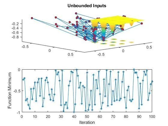
Figure 2:

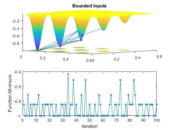
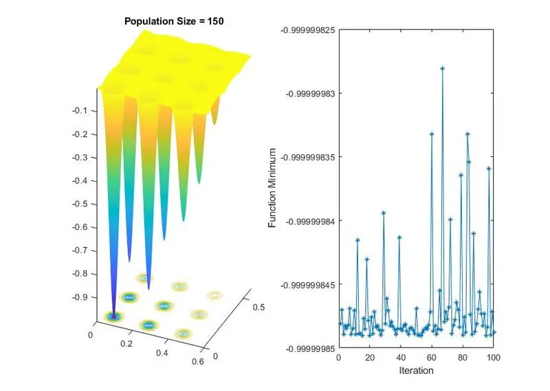
Figure 3:

Study time without bounds:3.8516

Study time with bounds:5.4619

Study time with higher population size:21.6706

In the third study, Roulette Wheel selection strategy is used and Adaptive Feasible Mutation strategy has been choosen based on the study of the references cited. After trial and error a Cross Over fraction of 0.4 and an Elite population size of 0.04*150 was found to give the best results.

The third study still has almost 2/150 that is about a 1.3% chance of ending up at a local minimum of -0.8. This was found by running the code repeatedly for 3-4 times. This is very small and may be neglected.

Hence, study 3 finally suggests that the global maxima of the function is 1 occuring at x = 0.0668 and y = 0.0668.

REFERENCES:

1. Youtube video: https://www.youtube.com/watch?v=MLPHLm56inQ for basic concepts

2. Matlab Documentation

3. Wikipedia

4. Soft Computing Applications by Dr. Debasis Samanta, course material (PDF)