Challenge

Week 5 - Curve fitting

AAnil Dubey3 Jun 2021

ANSWERS TO QUESTIONS ASKED

1. What does popt and pcov mean? (Watch the video to get some context)

Ans:
popt returns a list of suitable values of the constants for function 'func' passed as the first argument of curve_fit function. pcov returns a 2-D vector of covariance. It contains covariance of each coefficient of the function 'func' passed to the curve_fit with itself and also with other constants. Diagonal elements contain the covariance of each constant with itself.

2. What does np.array(temperature) do?

Ans:
Statement np.array(temperature) converts the python list, temperature to a numpy array.
This is important, otherwise the following error message will be raised if we try to multiply values in python list 'temperature' with the constants obtained from curve_fit (*popt):

TypeError: can't multiply sequence by non-int of type 'numpy.float64'

List is a heterogenous data structure (can store elements of multiple data types together in contiguous memory location) which need not be declared previously.Python core library provides list as a data structure.

An array is a data structure which stores values of same type in contiguous memory location. In Python arrays are implemented through Numpy arrays. Numpy is a core library for scientific computing in Python.

3. What does the * in *popt mean?

Ans:
The infix operator * stands for multiplication in Python. For exmample 2*3 will return 6 as output. As a unary prefix operator (an operator appearing before its operand) * is used to 'unpack' a list. Here also, popt stores the values of all the constants returned by curve_fit function and *popt 'unpacks' them to an argument list for constants in the function 'func" defining our polynomial.

4. Write code to fit a linear and cubic polynomial for the Cp data. Explain if your results are good or bad.

Ans:

'''
CURVE FITTING ASSIGNMENT BY ANIL DUBEY
'''

import matplotlib.pyplot as plt
import numpy as np
from scipy.optimize import curve_fit

#Curve-fit functions
def func_1(t, a, b):
    
    return a*t + b #Linear

def func_2(t, a, b, c):
   
    return a*pow(t,2) + b*t + c #Quadratic

def func_3(t, a, b, c, d):
    
    return a*pow(t,3) + b*pow(t,2) + c*t + d #Cubic

def func_4(t, a, b, c, d, e):
    
    return a*pow(t,4) + b*pow(t,3) + c*pow(t,2) + d*t + e #Quartic

#Performing the curve fitting
def CF(func,temp,cp):
    popt, pcov = curve_fit(func, temp, cp)
    fit_cp = func(np.array(temp), *popt)
    return fit_cp, popt, pcov

#Function to evaluate goodness of  fit
def GoF(t,cp,func, popt):
    
    print ("Mean Squared Error: ", np.mean((cp-func(np.array(t), *popt))**2))

    ss_res = np.dot((cp - func(np.array(t), *popt)),(cp - func(np.array(t), *popt)))
    ymean = np.mean(cp)
    ss_tot = np.dot((cp-ymean),(cp-ymean))
    print ("R-Square Value:",  1-ss_res/ss_tot)

#Function for Reading thermodynamic data file
def read_file():
    
    temperature = []
    cp = []
    
    for line in open('data', 'r'):
        values = line.split(',')
        temperature.append(float(values[0]))
        cp.append(float(values[1]))
    
    return [temperature,cp]

#Reading data from the file
temperature, cp = read_file()

#Attempting linear fit
fit_cp_linear, popt, pcov = CF(func_1, temperature, cp)
print('Goodness of fit for linear polynomial:')
GoF(temperature,cp,func_1,popt)
print()
#Attempting cubic fit
fit_cp_cubic, popt, pcov = CF(func_3, temperature, cp)
print('Goodness of fit for cubic polynomial:')
GoF(temperature,cp,func_3,popt)
print()

#Choosing different polynimials for different regions of the curve to obtain a better #fit
ind = temperature.index(1500.0)
temp1 = temperature[0:ind+1]
temp2 = temperature[ind+1:]
fit1, popt1, pcov1 = CF(func_4, temp1, cp[0:ind+1])
fit2, popt2, pcov2 = CF(func_2, temp2, cp[ind+1:])
print('Goodness of fit for temperature range %.1f to %.1f with quartic polynomial:'%(temperature[0],temperature[ind]))
GoF(temp1,cp[0:ind+1],func_4,popt1)
print()
print('Goodness of fit for temperature range %.1f to %.1f with quadratic polynomial:'%(temperature[ind+1],temperature[-1]))
GoF(temp2,cp[ind+1:],func_2,popt2)
print()

#The following lines of code disply the plots in the same window
#just like subplot function of Matlab
# with sharex and sharey the axes are shared among all the plots and inner axes labels #are removed
fig, ax = plt.subplots(2, 3, sharex = True, sharey = True)
fig.suptitle('CURVE FITTING')

ax[0,0].plot(temperature, cp, color  = 'blue', linewidth = 3)
ax[0,0].set_title('Original temp vs cp')

ax[0,1].plot(temperature, cp, color  = 'blue', linewidth = 3)
ax[0,1].plot(temperature, fit_cp_linear, color  = 'red', linewidth = 3)
ax[0,1].set_title('Linear fit')

ax[0,2].plot(temperature, cp, color  = 'blue', linewidth = 3)
ax[0,2].plot(temperature, fit_cp_cubic, color  = 'red', linewidth = 3)
ax[0,2].set_title('Cubic fit')

ax[1,0].plot(temperature, cp, color  = 'blue', linewidth = 3)
ax[1,0].plot(temp1, fit1, color  = 'red', linewidth = 3)
ax[1,0].set_title('Quartic fit for temp<1500')

ax[1,1].plot(temperature, cp, color  = 'blue', linewidth = 3)
ax[1,1].plot(temp2, fit2, color  = 'green', linewidth = 3)
ax[1,1].set_title('Quadratic fit for temp>1500')

ax[1,2].plot(temperature, cp, color  = 'blue', linewidth = 3)
ax[1,2].plot(temp1, fit1, color  = 'red', linewidth = 3)
ax[1,2].plot(temp2, fit2, color  = 'green', linewidth = 3)
ax[1,2].set_title('Quartic and Quadratic fits together')

#The following loop sets labels for all the axes
for A in ax.flat:
    A.set(xlabel = 'Temperature (K)', ylabel = 'Cp')

#The following loop ensures that only outer potion of axes are labelled
#Otherwise the plot will look too packed and ugly
for A in ax.flat:
    A.label_outer()
    

#The following two lines ensure that the figure opens in maximised state
mng = plt.get_current_fig_manager()
mng.window.state('zoomed') #works fine on Windows only

fig.show()
plt.savefig("Curve_fitting.jpeg",dpi=600)

The output was:

>>>

Goodness of fit for linear polynomial:
Mean Squared Error: 675.9528403686832
R-Square Value: 0.9248776260551824

Goodness of fit for cubic polynomial:
Mean Squared Error: 29.460006412729314
R-Square Value: 0.9967259467140538

Goodness of fit for temperature range 300.0 to 1500.0 with quartic polynomial:
Mean Squared Error: 1.343476770560602
R-Square Value: 0.9997174708061651

Goodness of fit for temperature range 1501.0 to 3499.0 with quadratic polynomial:
Mean Squared Error: 0.2769264992105013
R-Square Value: 0.9998290863891499

Explanation:

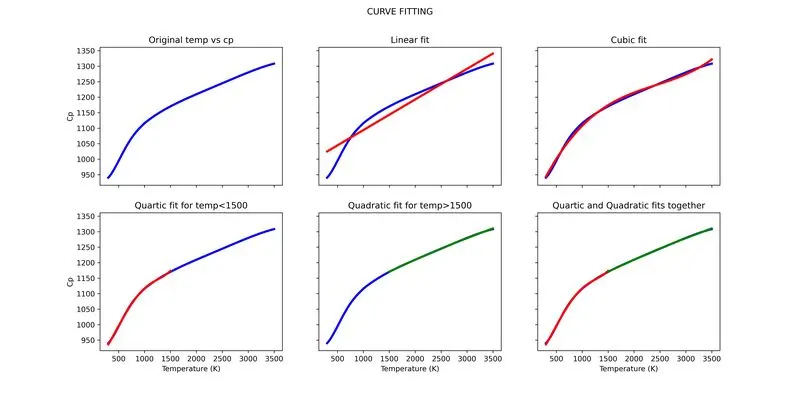
Now, as we can see that the Mean Squared Error is lesser for cubic fit as compared to the linear fit. So, cubic fit is better. The R-squared value is also better (more close to 1.0) in the case of cubic fit. The drawback of using only R-Squared value is that even for a linear fit which is nowhere close to representing the actual data the R-Squared value is very close to 1 i.e. 0.924. So it is better to use multiple parameters to ascertain the goodness of fit.

The following plot was obtained through the above code:

5. What needs to be done in order to make the curve fit perfect?

Ans:

To make the fit perfect the following could be done:
a. Increasing the order of the polynomial: Using a quartic polynomial may lead to a better fit than cubic fit.

b. Using two different curves for two different parts of the data set: After trial and error with the above code it was found that a nearly perfect fit for the above data set is obtained if we choose a quartic (4th order polynomial) for temperature less than 1500 K and a quadratic polynomial for temperature more than 1500 K. Kindly, refer to the figure attached with the previous answer.

6. Show empirically how well your curve has been fit.

Ans:
In order to empirically assess the goodness of fit the following two parameters have been calculated.

a. Mean Squared Error- It is the mean/average of the square of the difference between the actual data and the curve fit. The closer is the value to 0, the better is the curve-fit
b. R-Square Value- It is the ratio of sum of square of the regression (SSR) to that of the total sum of square (SST). Sum of square of the regression is nothing but
sum of the square of the difference between the value obtained from the curve fit and the mean of the actual data. Total sum of square is the sum of the square of the difference
between actual data values and mean of the actual data values. The closer is the R-Square value to 1 the better is the curve fit.

The corresponding values for the above goodness of fit parameters were presented in the answer to question no 4, and have been again presented below for the convenience of the reader.